Air separation modeling. — bdrworks.org Handbook

Question

A plant needs gaseous nitrogen at 8 bar with at most 1 ppm of oxygen. (1) At what temperatures does air condense, and at what pressures must the two columns of a double-column plant run? (2) How much nitrogen can a single cryogenic column at 8 bar deliver at that purity, and where does the argon of the air go? (3) What could a membrane unit deliver instead, and how do the energy needs of the three routes compare with the thermodynamic minimum?

1The problem

Dry air contains about 78.1 % nitrogen, 20.9 % oxygen and 0.93 % argon by volume (U.S. Standard Atmosphere, 1976; Häussinger et al., 2000a, Sec. 3). Nitrogen for inerting, chemicals and electronics is obtained by separating it, and three technologies compete: cryogenic rectification, pressure-swing adsorption on carbon molecular sieves and polymer membranes. Which one is cheapest depends on the purity and the capacity required; cryogenic plants dominate at high purity and large flows, adsorption and membranes at lower purity and small flows (Häussinger et al., 2000a, Sec. 4 and Fig. 3).

This page follows the Ullmann article on nitrogen through the three routes (Häussinger et al., 2000a, Secs. 4.1–4.3). Each solution is written in Python and in MATLAB; the two versions give the same numbers, and the MATLAB files also run in GNU Octave.

2Ways to separate air

Rectification needs a liquid, and air can only be liquefied below its critical point, about 132.5 K and 37.7 bar. Cooling one kilogram of air from +15 to −196 °C removes about 415 kJ; the refrigeration comes from Joule–Thomson throttling or, more effectively, from expansion turbines, and the air is precooled in counter-current heat exchangers against the cold products (Häussinger et al., 2000a, Sec. 4.1). Before it is cooled the compressed air passes zeolite adsorbers that remove water, carbon dioxide and hydrocarbons, which would otherwise freeze out (Häussinger et al., 2000a, Sec. 4.1).

The simplest cryogenic plant is the single-column nitrogen generator: air enters the bottom of a column at 6–10 bar, pure nitrogen leaves the top, and oxygen-enriched liquid collects at the bottom. Part of the top nitrogen is the product; the rest is condensed as reflux against the bottom liquid, which is throttled and evaporated in the same heat exchanger and then expanded in a turbine to provide the cold (Häussinger et al., 2000a, Sec. 4.1 and Fig. 5). When oxygen is also wanted, a double column is used: a high-pressure (HP) column preseparates the air, and a low-pressure (LP) column on top of it produces pure oxygen at the bottom and pure nitrogen at the top. The condenser of the HP column is the reboiler of the LP column, which fixes the ratio of the two pressures (Häussinger et al., 2000a, Sec. 4.1, Figs. 4 and 6).

Pressure-swing adsorption uses carbon molecular sieves that take up oxygen faster than nitrogen; air at 5–12 bar gives nitrogen with down to 100 ppm O₂, or less than 10 ppm with newer sieves (Häussinger et al., 2000a, Sec. 4.2). Membranes separate by solution and diffusion in a dense polymer skin, and practically all polymers pass oxygen faster than nitrogen, so the nitrogen product is the retentate (Häussinger et al., 2000a, Sec. 4.3 and Table 6; Strathmann, 2005, Sec. 4).

3Thermodynamic data

Nitrogen, argon and oxygen are simple, non-polar molecules, so a corresponding-states correlation predicts their vapour pressures well. The Lee–Kesler correlation is used, with the critical constants of Smith et al. and an acentric factor that reproduces the normal boiling point, as Lee and Kesler recommend (Lee & Kesler, 1975; Smith et al., 2018, Eqs. 6.92–6.95 and Table B.1):

$$\begin{gathered}\ln P_r^{sat} = \ln P_r^{0}(T_r) + \omega\,\ln P_r^{1}(T_r) \\[6pt] \ln P_r^{0} = 5.92714 - \frac{6.09648}{T_r} - 1.28862\ln T_r + 0.169347\,T_r^6 \\[4pt] \ln P_r^{1} = 15.2518 - \frac{15.6875}{T_r} - 13.4721\ln T_r + 0.43577\,T_r^6\end{gathered}$$Eq. 1 — Lee–Kesler vapour pressure

Against the measured saturation pressures of nitrogen tabulated by Häussinger et al. it is within 0.6 % from the triple point (63.15 K) to 120 K (Häussinger et al., 2000a, Table 1). Liquid air is not far from an ideal solution and the gas is nearly ideal at these pressures, so Raoult's law gives a first model of the phase equilibrium (Smith et al., 2018, Sec. 13.3, Eqs. 13.16–13.19):

$$y_i\,P = x_i\,P_i^{sat}(T), \qquad K_i = \frac{P_i^{sat}}{P}, \qquad \text{dew: } \sum_i \frac{y_i}{K_i} = 1, \qquad \text{bubble: } \sum_i K_i\,x_i = 1$$Eq. 2 — Raoult’s law

Latent heats follow from the Clapeyron equation, with the vapour and liquid volumes from the Peng–Robinson equation (Smith et al., 2018, Eq. 4.12 and Sec. 3.6; Peng & Robinson, 1976):

$$\Delta H^{lv} = T\,\Delta V^{lv}\,\frac{dP^{sat}}{dT} = R\,T^2\,(Z^v - Z^l)\,\frac{d\ln P^{sat}}{dT}$$Eq. 3 — Clapeyron equation

For nitrogen it gives 5.52 kJ/mol at 80 K and 4.48 kJ/mol at 100 K, against 5.47 and 4.50 kJ/mol from the enthalpies of Table 1 of Häussinger et al. (Häussinger et al., 2000a, Table 1). Carbon dioxide and water are removed before the cold box and the small amounts of neon, helium and krypton are neglected, so air is treated as the ternary N₂–Ar–O₂ (U.S. Standard Atmosphere, 1976).

4Solution 1 · Liquefying air and the double column

With Eq. 2 the dew point of air, where the first drop forms, and its bubble point, where the last vapour condenses, are found with a one-dimensional root search at each pressure (Brent, 1973; Finlayson et al., 2006, Sec. 1.3).

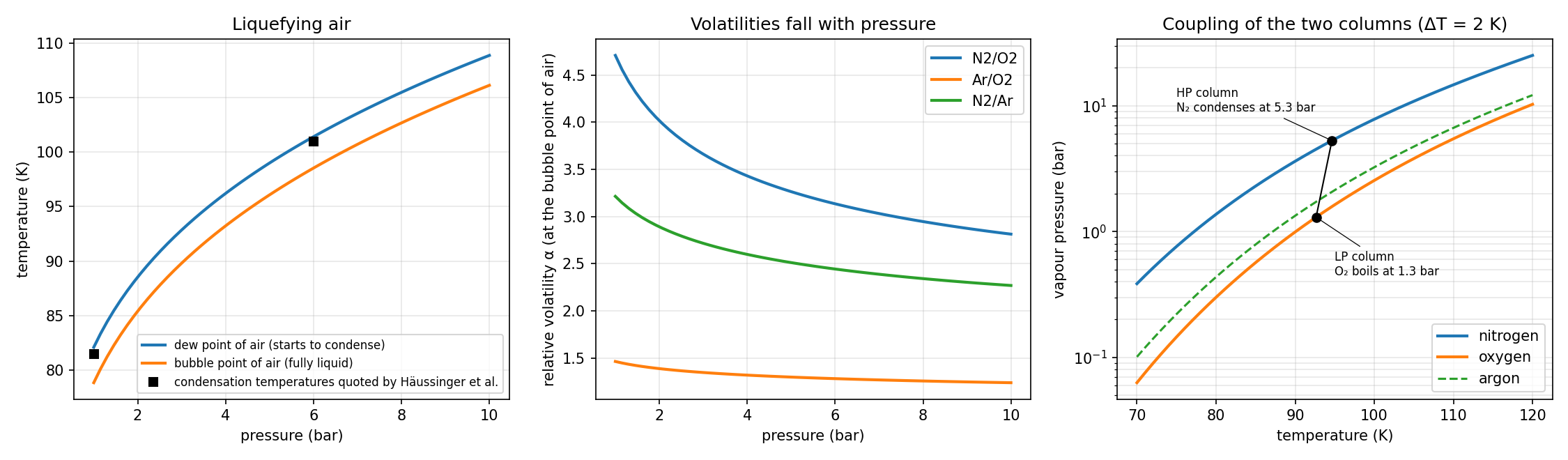
**Figure 1.** Left: dew and bubble points of air against pressure, with the condensation temperatures quoted by Häussinger et al. Middle: relative volatilities at the bubble point of air. Right: vapour pressures of nitrogen, argon and oxygen, and the coupling of the two columns for a 2 K temperature difference in the main condenser.

Air starts to condense at 82.1 K at 1 bar and at 101.4 K at 6 bar; Häussinger et al. quote 81.5 and 101 K (Häussinger et al., 2000a, Sec. 4.1). Because air is a mixture it condenses over a range of about 3 K. Two results from the middle panel shape every cryogenic plant:

Nitrogen is much more volatile than oxygen, but the relative volatility falls from 4.7 at 1 bar to 2.9 at 8 bar. Separation is easier at low pressure, which is why the final, sharp separation of a double column is made in the LP column (Häussinger et al., 2000a, Sec. 4.1).
Argon lies between the two, and it is only 1.3–1.5 times as volatile as oxygen. It is difficult to separate from oxygen and it accumulates in the middle of a column, which Solution 2 shows.

The right panel shows the coupling of a double column. Oxygen boils in the sump of the LP column at about 1.3 bar and 92.6 K. The nitrogen at the top of the HP column must condense against it, and with a temperature difference of about 2 K for heat transfer it must condense at 94.6 K, which requires 5.3 bar (Häussinger et al., 2000a, Sec. 4.1 and Fig. 4). A difference of 1 to 2.5 K moves the HP pressure between 4.9 and 5.5 bar: the main condenser, not the choice of the designer, sets the air compressor pressure. The latent heat of oxygen at the LP pressure is also larger than that of nitrogen at the HP pressure, 6.79 against 4.81 kJ/mol, so each mole of nitrogen condensed evaporates only 0.71 mol of oxygen.

Air (N₂–Ar–O₂)	1 bar	6 bar	8 bar
Dew point	82.11 K	101.41 K	105.47 K
Bubble point	78.86 K	98.54 K	102.67 K
α N₂/O₂ at the bubble point	4.71	3.13	2.95
α Ar/O₂ at the bubble point	1.46	1.28	1.26

Raoult's law is the weakest part of this model. Near the sump of an LP column it gives volatilities of nitrogen, argon and oxygen in the ratio 3.5 : 1.3 : 1, against 3.6 : 1.5 : 1 quoted for such a column in the Ullmann article on the noble gases, and for argon dissolved in nitrogen at 6 bar it gives K_Ar = 0.40 where that article gives 0.54 (Häussinger et al., 2000b, Sec. 4.1.2). The nitrogen–oxygen split is described well, but argon is more volatile in liquid nitrogen than an ideal solution allows, so an activity-coefficient model is needed for quantitative argon work (Smith et al., 2018, Sec. 13.4).

air_equilibrium.pyDownload

"""
Air separation — phase equilibrium of air and the pressures of a double column
bdrworks.org · Handbook · Air separation, worked model 1

Vapour pressures of N2, Ar and O2 from the Lee–Kesler corresponding-states correlation,
    ln Pr_sat = ln Pr0(Tr) + w ln Pr1(Tr),  w fitted to the normal boiling point,
and Raoult's law K_i = Psat_i/P for the ternary N2–Ar–O2 (CO2 and water are removed upstream).
Dew and bubble points of air follow from sum(y/K) = 1 and sum(K x) = 1.
Latent heats come from the Clapeyron equation, dH = T dV dPsat/dT, with the vapour and liquid
volumes of the Peng–Robinson equation (check against measured nitrogen data).
The double column couples the two pressures: nitrogen condensing in the HP column must be
dT (about 2 K) warmer than oxygen boiling in the LP column.

Run:  python air_equilibrium.py      (needs numpy, scipy, matplotlib)
"""
import numpy as np
from scipy.optimize import brentq
import matplotlib.pyplot as plt

RG = 8.314462618
SP = ["N2", "Ar", "O2"]
# Tc (K), Pc (bar), normal boiling point Tn (K), omega (for Peng–Robinson)
CRIT = {"N2": (126.2, 34.00, 77.35, 0.038), "Ar": (150.9, 48.98, 87.3, 0.000), "O2": (154.6, 50.43, 90.2, 0.022)}
AIR = np.array([0.78118, 0.00934, 0.20957]); AIR /= AIR.sum()        # dry, CO2-free air


def lnPr0(Tr):
    return 5.92714 - 6.09648/Tr - 1.28862*np.log(Tr) + 0.169347*Tr**6


def lnPr1(Tr):
    return 15.2518 - 15.6875/Tr - 13.4721*np.log(Tr) + 0.43577*Tr**6


# Lee–Kesler acentric factor that reproduces the normal boiling point
W_LK = {s: (np.log(1.01325/CRIT[s][1]) - lnPr0(CRIT[s][2]/CRIT[s][0]))/lnPr1(CRIT[s][2]/CRIT[s][0]) for s in SP}


def psat(s, T):
    Tc, Pc = CRIT[s][:2]
    Tr = T/Tc
    return Pc*np.exp(lnPr0(Tr) + W_LK[s]*lnPr1(Tr))                  # bar


def tsat(s, P):
    return brentq(lambda T: psat(s, T) - P, 50.0, CRIT[s][0] - 1e-6)


def K(T, P):
    return np.array([psat(s, T) for s in SP])/P


def dew_T(y, P):
    return brentq(lambda T: (y/K(T, P)).sum() - 1.0, 55.0, 150.0)


def bubble_T(x, P):
    return brentq(lambda T: K(T, P) @ x - 1.0, 55.0, 150.0)


def pr_volumes(s, T, P):
    """Liquid and vapour compressibility factors from Peng–Robinson (P in bar)."""
    Tc, Pc, _, w = CRIT[s]
    kap = 0.37464 + 1.54226*w - 0.26992*w*w
    a = 0.45724*(RG*Tc)**2/(Pc*1e5)*(1 + kap*(1 - np.sqrt(T/Tc)))**2
    b = 0.07780*RG*Tc/(Pc*1e5)
    A, B = a*P*1e5/(RG*T)**2, b*P*1e5/(RG*T)
    r = np.roots([1.0, -(1 - B), A - 3*B*B - 2*B, -(A*B - B*B - B**3)])
    r = np.sort(r[np.abs(r.imag) < 1e-10].real)
    return r[0], r[-1]


def latent_heat(s, T):
    """Clapeyron: dH = R T^2 (Zv - Zl) dln(Psat)/dT, J/mol."""
    h = 1e-3
    dlnP = (np.log(psat(s, T + h)) - np.log(psat(s, T - h)))/(2*h)
    zl, zv = pr_volumes(s, T, psat(s, T))
    return RG*T*T*(zv - zl)*dlnP


if __name__ == "__main__":
    print("Lee–Kesler omega:", {s: round(W_LK[s], 4) for s in SP})
    print("Nitrogen vapour pressure against measured data (Ullmann, Nitrogen, Table 1):")
    for T, P_meas in [(63.15, 0.1246), (80, 1.367), (100, 7.777), (120, 25.13)]:
        print(f"  {T:6.2f} K: {psat('N2', T):7.4f} bar vs {P_meas} bar ({100*(psat('N2', T)/P_meas - 1):+.2f} %)")
    for T, dH_meas in [(80, 2218.0 + 3248.0), (100, 2466.0 + 2033.0), (120, 2103.0 + 504.6)]:
        print(f"  latent heat {T} K: {latent_heat('N2', T):.0f} J/mol vs {dH_meas:.0f} J/mol")
    print("normal boiling points:", {s: round(tsat(s, 1.01325), 2) for s in SP})
    for P in [1.0, 6.0, 8.0]:
        print(f"air at {P:.0f} bar: dew point {dew_T(AIR, P):.2f} K, bubble point {bubble_T(AIR, P):.2f} K")

    # double column: O2 boils in the LP sump, N2 condenses at the HP top
    PL = 1.3
    TO2 = tsat("O2", PL)
    for dT in [1.0, 1.5, 2.0, 2.5]:
        print(f"LP {PL} bar (O2 boils at {TO2:.2f} K), dT = {dT} K -> HP column at {psat('N2', TO2 + dT):.2f} bar")
    print(f"latent heats in the main condenser: N2 at HP {latent_heat('N2', TO2 + 2):.0f} J/mol, O2 at LP {latent_heat('O2', TO2):.0f} J/mol")

    fig, ax = plt.subplots(1, 3, figsize=(15, 4.4))
    Ps = np.linspace(1.0, 10.0, 60)
    ax[0].plot(Ps, [dew_T(AIR, P) for P in Ps], lw=2, label="dew point of air (starts to condense)")
    ax[0].plot(Ps, [bubble_T(AIR, P) for P in Ps], lw=2, label="bubble point of air (fully liquid)")
    ax[0].plot([1.0, 6.0], [81.5, 101.0], "ks", label="condensation temperatures quoted by Häussinger et al.")
    ax[0].set(xlabel="pressure (bar)", ylabel="temperature (K)", title="Liquefying air")
    ax[0].legend(fontsize=8); ax[0].grid(alpha=0.3)

    for pair, c in [(("N2", "O2"), "tab:blue"), (("Ar", "O2"), "tab:orange"), (("N2", "Ar"), "tab:green")]:
        al = [psat(pair[0], bubble_T(AIR, P))/psat(pair[1], bubble_T(AIR, P)) for P in Ps]
        ax[1].plot(Ps, al, lw=2, color=c, label=f"{pair[0]}/{pair[1]}")
    ax[1].set(xlabel="pressure (bar)", ylabel="relative volatility α (at the bubble point of air)", title="Volatilities fall with pressure")
    ax[1].legend(); ax[1].grid(alpha=0.3)

    Ts = np.linspace(70, 120, 200)
    ax[2].semilogy(Ts, [psat("N2", T) for T in Ts], lw=2, label="nitrogen")
    ax[2].semilogy(Ts, [psat("O2", T) for T in Ts], lw=2, label="oxygen")
    ax[2].semilogy(Ts, [psat("Ar", T) for T in Ts], lw=1.5, ls="--", label="argon")
    PH = psat("N2", TO2 + 2.0)
    ax[2].plot([TO2, TO2 + 2.0], [PL, PH], "k-", lw=1)
    ax[2].plot([TO2], [PL], "ko"); ax[2].plot([TO2 + 2.0], [PH], "ko")
    ax[2].annotate(f"LP column\nO₂ boils at {PL} bar", (TO2, PL), xytext=(95, 0.45), fontsize=8, arrowprops=dict(arrowstyle="-", lw=0.6))
    ax[2].annotate(f"HP column\nN₂ condenses at {PH:.1f} bar", (TO2 + 2.0, PH), xytext=(75, 9), fontsize=8, arrowprops=dict(arrowstyle="-", lw=0.6))
    ax[2].set(xlabel="temperature (K)", ylabel="vapour pressure (bar)", title="Coupling of the two columns (ΔT = 2 K)")
    ax[2].legend(loc="lower right"); ax[2].grid(alpha=0.3, which="both")
    fig.tight_layout(); fig.savefig("air_equilibrium.png", dpi=150)
    plt.show()

air_equilibrium.mDownload

function air_equilibrium()
% Air separation - phase equilibrium of air and the pressures of a double column
% bdrworks.org - Handbook - Air separation, worked model 1
%   Lee-Kesler vapour pressures (omega fitted to the normal boiling point), Raoult's law,
%   dew and bubble points of N2-Ar-O2 air, Clapeyron latent heats with Peng-Robinson volumes
% Save as air_equilibrium.m and run:  air_equilibrium      (MATLAB or GNU Octave)

air = [0.78118; 0.00934; 0.20957];  air = air/sum(air);         % N2, Ar, O2
fprintf('Lee-Kesler omega: N2 %.4f, Ar %.4f, O2 %.4f\n', wlk(1), wlk(2), wlk(3));
Tm = [63.15 80 100 120];  Pm = [0.1246 1.367 7.777 25.13];
for k = 1:4
    fprintf('  N2 %6.2f K: %7.4f bar vs %.4f bar (%+.2f %%)\n', Tm(k), psat(1, Tm(k)), Pm(k), 100*(psat(1, Tm(k))/Pm(k) - 1));
end
Hm = [2218+3248, 2466+2033, 2103+504.6];
for k = 1:3
    fprintf('  latent heat %d K: %.0f J/mol vs %.0f J/mol\n', Tm(k+1), latent(1, Tm(k+1)), Hm(k));
end
for P = [1 6 8]
    fprintf('air at %d bar: dew point %.2f K, bubble point %.2f K\n', P, dewT(air, P), bubT(air, P));
end
PL = 1.3;  TO2 = tsat(3, PL);
for dT = [1 1.5 2 2.5]
    fprintf('LP %.1f bar (O2 boils at %.2f K), dT = %.1f K -> HP column at %.2f bar\n', PL, TO2, dT, psat(1, TO2 + dT));
end
fprintf('latent heats in the main condenser: N2 at HP %.0f J/mol, O2 at LP %.0f J/mol\n', latent(1, TO2 + 2), latent(3, TO2));

Ps = linspace(1, 10, 40);
figure('Position', [60 100 1300 380]);
subplot(1,3,1);
plot(Ps, arrayfun(@(p) dewT(air, p), Ps), Ps, arrayfun(@(p) bubT(air, p), Ps), 'LineWidth', 2); hold on;
plot([1 6], [81.5 101], 'ks');
xlabel('pressure (bar)'); ylabel('temperature (K)'); title('Liquefying air'); legend('dew point', 'bubble point', 'quoted values'); grid on;
subplot(1,3,2);
aNO = arrayfun(@(p) psat(1, bubT(air, p))/psat(3, bubT(air, p)), Ps);
aAO = arrayfun(@(p) psat(2, bubT(air, p))/psat(3, bubT(air, p)), Ps);
plot(Ps, aNO, Ps, aAO, 'LineWidth', 2);
xlabel('pressure (bar)'); ylabel('relative volatility'); title('Volatilities fall with pressure'); legend('N_2/O_2', 'Ar/O_2'); grid on;
subplot(1,3,3);
Ts = linspace(70, 120, 100);
semilogy(Ts, arrayfun(@(t) psat(1, t), Ts), Ts, arrayfun(@(t) psat(3, t), Ts), 'LineWidth', 2); hold on;
semilogy([TO2 TO2+2], [PL psat(1, TO2+2)], 'ko-');
xlabel('temperature (K)'); ylabel('vapour pressure (bar)'); title('Coupling of the two columns'); legend('N_2', 'O_2'); grid on;
end

% ---------------------------------------------------------------- property model
function c = crit()
% Tc (K), Pc (bar), Tn (K), omega (Peng-Robinson): N2, Ar, O2
c = [126.2 34.00 77.35 0.038; 150.9 48.98 87.3 0.000; 154.6 50.43 90.2 0.022];
end

function v = lnPr0(Tr),  v = 5.92714 - 6.09648./Tr - 1.28862*log(Tr) + 0.169347*Tr.^6;  end
function v = lnPr1(Tr),  v = 15.2518 - 15.6875./Tr - 13.4721*log(Tr) + 0.43577*Tr.^6;  end

function w = wlk(i)
c = crit();  Trn = c(i,3)/c(i,1);
w = (log(1.01325/c(i,2)) - lnPr0(Trn))/lnPr1(Trn);
end

function p = psat(i, T)
c = crit();  Tr = T/c(i,1);
p = c(i,2)*exp(lnPr0(Tr) + wlk(i)*lnPr1(Tr));
end

function T = tsat(i, P)
c = crit();  T = fzero(@(t) psat(i, t) - P, [50 c(i,1) - 1e-6]);
end

function k = Kv(T, P),  k = [psat(1, T); psat(2, T); psat(3, T)]/P;  end
function T = dewT(y, P),  T = fzero(@(t) sum(y./Kv(t, P)) - 1, [55 150]);  end
function T = bubT(x, P),  T = fzero(@(t) sum(Kv(t, P).*x) - 1, [55 150]);  end

function L = latent(i, T)
% Clapeyron with Peng-Robinson vapour and liquid compressibility factors, J/mol
R = 8.314462618;  c = crit();  P = psat(i, T);
kap = 0.37464 + 1.54226*c(i,4) - 0.26992*c(i,4)^2;
a = 0.45724*(R*c(i,1))^2/(c(i,2)*1e5)*(1 + kap*(1 - sqrt(T/c(i,1))))^2;  b = 0.07780*R*c(i,1)/(c(i,2)*1e5);
A = a*P*1e5/(R*T)^2;  B = b*P*1e5/(R*T);
z = roots([1, -(1 - B), A - 3*B^2 - 2*B, -(A*B - B^2 - B^3)]);  z = sort(real(z(abs(imag(z)) < 1e-10)));
h = 1e-3;  dlnP = (log(psat(i, T + h)) - log(psat(i, T - h)))/(2*h);
L = R*T^2*(z(end) - z(1))*dlnP;
end

5Solution 2 · Single-column nitrogen generator

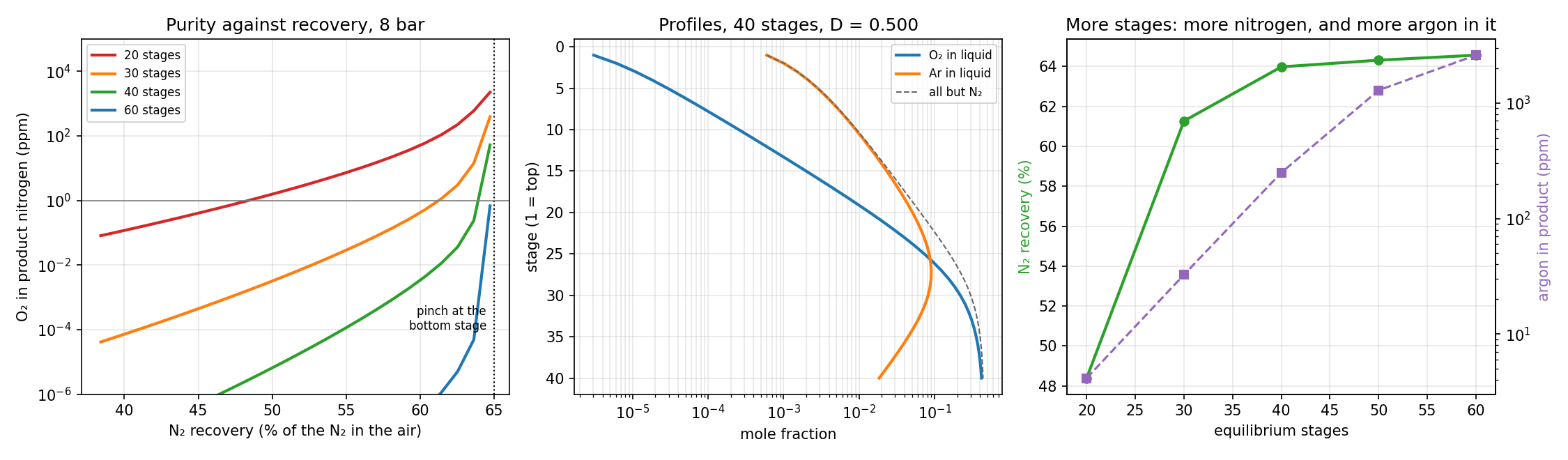
The column of Ullmann's Fig. 5 is modelled as N equilibrium stages at 8 bar, numbered from the top. The purified air enters below the bottom stage as saturated vapour; the vapour leaving the top stage is split into the gaseous product D and the part that is condensed and returned as reflux (Häussinger et al., 2000a, Sec. 4.1 and Fig. 5). With constant molar overflow the vapour flow is the feed, V = 1, and the liquid flow is L = 1 − D on every stage (Walas, 1990, Sec. 13.10; Walas, 1990, Sec. 13.4). The component balances on each stage are then:

$$\begin{gathered}L\,x_{i,j-1} + V\,y_{i,j+1} - L\,x_{i,j} - V\,y_{i,j} = 0, \qquad y_{i,j} = K_{i,j}\,x_{i,j} \\[6pt] L\,x_{i,j-1} - (L + V K_{i,j})\,x_{i,j} + V K_{i,j+1}\,x_{i,j+1} = 0\end{gathered}$$Eq. 4 — stage balances, a tridiagonal system for each component

For fixed stage temperatures these are linear, and for each component they form a tridiagonal system that is solved directly with the Thomas algorithm (Walas, 1990, Sec. 13.10, Eq. 13.193; Finlayson et al., 2006, Sec. 1.2). The liquid mole fractions are then normalised and each stage temperature is replaced by the bubble point of its liquid, found by Newton's method; this is the bubble-point method of Wang and Henke (Wang & Henke, 1966; Walas, 1990, Sec. 13.10 and Fig. 13.17). Close to the pinch the plain iteration oscillates, so the temperature update is damped whenever the correction grows.

There is an upper limit to the product that no number of stages can overcome. The bottom liquid cannot be richer in oxygen than the liquid in equilibrium with the air feed, so the oxygen balance fixes the largest product flow:

$$x_{i}^{*} = \frac{z_i}{K_i(T_{dew})}, \qquad D_{max} = 1 - \frac{z_{O_2}}{x_{O_2}^{*}}$$Eq. 5 — pinch at the bottom stage

At 8 bar this liquid contains 42.6 % O₂, and D_max = 0.508 mol per mol of air, or 65 % of the nitrogen in the air. The rest leaves with the oxygen-rich bottom liquid as residual gas.

**Figure 2.** Left: oxygen in the product against nitrogen recovery for 20 to 60 equilibrium stages; the dotted line is the pinch. Middle: oxygen and argon in the liquid on each stage for 40 stages at 1 ppm O₂. Right: recovery and argon content of the product at 1 ppm O₂ against the number of stages.

Stages (8 bar, 1 ppm O₂)	D (mol/mol air)	N₂ recovery	Ar in product	Bottom liquid O₂
20	0.378	48.4 %	4 ppm	33.7 %
30	0.479	61.3 %	33 ppm	40.2 %
40	0.500	64.0 %	249 ppm	41.9 %
60	0.506	64.6 %	2600 ppm	42.4 %

Three points stand out:

Purity is cheap and recovery is expensive. Every ten stages lower the oxygen content by two to three orders of magnitude at the same recovery, but beyond about 40 stages the recovery can only creep towards the 65 % pinch. Commercial single-column plants deliver nitrogen with about 1 ppm O₂ (Häussinger et al., 2000a, Sec. 4.1).
Argon goes with the nitrogen. Its concentration peaks at about 9 % in the middle of the column, where it is squeezed between the more volatile nitrogen and the less volatile oxygen. The more nitrogen is taken off at the top, the more argon it carries: from 4 ppm at 20 stages to 0.26 % at 60 stages. This is why Ullmann notes that the product of such plants contains argon besides the trace of oxygen (Häussinger et al., 2000a, Sec. 4.1). In oxygen plants the same maximum, up to 15 % argon in the vapour of the LP column, is where the side stream for the crude-argon column is drawn off (Häussinger et al., 2000b, Sec. 4.1.2). Because Raoult's law underestimates the volatility of argon in nitrogen (Solution 1), the argon contents in the table are lower bounds.
The condenser sets the residual-gas pressure. Nitrogen condenses at 100.4 K at the top; with a 2 K approach the bottom liquid, 41.9 % O₂, must fully evaporate at or below 3.6 bar, and this residual gas drives the expansion turbine (Häussinger et al., 2000a, Sec. 4.1).

The constant-molar-overflow model does not close the heat balance of the condenser: the latent heats of Solution 1 show that the condensing nitrogen supplies somewhat less heat than the evaporating bottom liquid needs. A model with full enthalpy balances, such as the sum-rates method, is needed for that (Walas, 1990, Sec. 13.10).

air_column.pyDownload

"""
Air separation — single-column nitrogen generator (cryogenic)
bdrworks.org · Handbook · Air separation, worked model 2

Purified air (saturated vapour, N2–Ar–O2) enters below the bottom stage of a column at 8 bar.
Nitrogen vapour leaves the top stage; the product D is taken as gas and the rest is condensed
against the evaporating bottom liquid and returned as reflux. The O2-rich bottom liquid is
throttled and evaporated in that condenser (residual gas, later expanded in a turbine).

Equilibrium-stage model with constant molar overflow (V = F = 1, L = 1 - D on every stage),
Raoult's law K-values from Lee–Kesler vapour pressures, solved with the Wang–Henke
bubble-point method: for fixed stage temperatures the component balances form a
tridiagonal system (Thomas algorithm); new temperatures are the bubble points.

Run:  python air_column.py      (needs numpy, scipy, matplotlib)
"""
import numpy as np
from scipy.optimize import brentq
import matplotlib.pyplot as plt

RG = 8.314462618
SP = ["N2", "Ar", "O2"]
CRIT = {"N2": (126.2, 34.00, 77.35), "Ar": (150.9, 48.98, 87.3), "O2": (154.6, 50.43, 90.2)}
AIR = np.array([0.78118, 0.00934, 0.20957]); AIR /= AIR.sum()


def lnPr0(Tr):
    return 5.92714 - 6.09648/Tr - 1.28862*np.log(Tr) + 0.169347*Tr**6


def lnPr1(Tr):
    return 15.2518 - 15.6875/Tr - 13.4721*np.log(Tr) + 0.43577*Tr**6


W_LK = {s: (np.log(1.01325/CRIT[s][1]) - lnPr0(CRIT[s][2]/CRIT[s][0]))/lnPr1(CRIT[s][2]/CRIT[s][0]) for s in SP}


def psat(s, T):
    Tc, Pc = CRIT[s][:2]
    return Pc*np.exp(lnPr0(T/Tc) + W_LK[s]*lnPr1(T/Tc))


def K(T, P):
    return np.array([psat(s, T) for s in SP])/P


def dlnpsat(s, T):
    """d ln Psat / dT of the Lee–Kesler correlation, 1/K."""
    Tc = CRIT[s][0]; Tr = T/Tc
    d0 = 6.09648/Tr**2 - 1.28862/Tr + 6*0.169347*Tr**5
    d1 = 15.6875/Tr**2 - 13.4721/Tr + 6*0.43577*Tr**5
    return (d0 + W_LK[s]*d1)/Tc


def Kmat(T, P):
    """K-values for a vector of stage temperatures: array (stages x 3)."""
    return np.column_stack([psat(s, T) for s in SP])/P


def bubble_T(X, P, T0):
    """Bubble points of all stages at once: Newton's method on ln(sum K x) = 0."""
    T = np.array(T0, dtype=float)
    for _ in range(60):
        Km = Kmat(T, P); s = (Km*X).sum(axis=1)
        dlog = (Km*X*np.column_stack([dlnpsat(sp, T) for sp in SP])).sum(axis=1)/s
        dT = np.clip(-np.log(s)/dlog, -10.0, 10.0)
        T = T + dT
        if np.abs(dT).max() < 1e-11:
            break
    return T


def dew_T(y, P):
    return brentq(lambda T: (y/K(T, P)).sum() - 1.0, 55.0, 150.0)


def thomas(a, b, c, d):
    """Solve a tridiagonal system (a: sub-, b: main, c: super-diagonal)."""
    n = len(d); cp = np.zeros(n); dp = np.zeros(n)
    cp[0], dp[0] = c[0]/b[0], d[0]/b[0]
    for i in range(1, n):
        m = b[i] - a[i]*cp[i - 1]
        cp[i] = c[i]/m if i < n - 1 else 0.0
        dp[i] = (d[i] - a[i]*dp[i - 1])/m
    x = np.zeros(n); x[-1] = dp[-1]
    for i in range(n - 2, -1, -1):
        x[i] = dp[i] - cp[i]*x[i + 1]
    return x


def column(N, D, P, z=AIR, tol=1e-9, itmax=3000):
    """N equilibrium stages (1 = top), vapour feed F = 1 below stage N, gaseous product D.
    Returns stage temperatures T, liquid x and vapour y (N x 3)."""
    L = 1.0 - D
    T = np.full(N, dew_T(z, P)); w, dT_old = 1.0, np.inf
    for it in range(itmax):
        Kj = Kmat(T, P)
        X = np.zeros((N, 3))
        for i in range(3):
            a = np.full(N, L); a[0] = 0.0
            b = -(L + Kj[:, i]); b[0] = -(L + D*Kj[0, i])    # top: reflux = condensed top vapour
            c = np.zeros(N); c[:-1] = Kj[1:, i]
            d = np.zeros(N); d[-1] = -z[i]
            X[:, i] = thomas(a, b, c, d)
        X = np.maximum(X, 1e-300)
        X /= X.sum(axis=1, keepdims=True)
        Tn = bubble_T(X, P, T)
        dT = np.abs(Tn - T).max()
        if dT < tol:
            T = Tn
            break
        if it > 0 and dT > dT_old:                      # oscillating near the pinch: damp the update
            w = max(0.5*w, 0.05)
        T, dT_old = T + w*(Tn - T), dT
    else:
        raise RuntimeError(f"no convergence for N = {N}, D = {D}")
    Y = Kmat(T, P)*X
    return T, X, Y


def pinch_D(P, z=AIR):
    """Largest product with no O2 in it: bottom liquid in equilibrium with the air feed."""
    Td = dew_T(z, P)
    xs = z/K(Td, P); xs /= xs.sum()
    return 1.0 - z[2]/xs[2], xs


def D_for_ppm(N, P, ppm=1.0):
    """Largest product flow that still meets the O2 specification (capped just below the pinch)."""
    f = lambda D: np.log(column(N, D, P)[2][0, 2]*1e6/ppm)
    Dhi = pinch_D(P)[0] - 0.002
    return Dhi if f(Dhi) < 0 else brentq(f, 0.20, Dhi, xtol=1e-6)


if __name__ == "__main__":
    P = 8.0
    Dmax, xs = pinch_D(P)
    print(f"pinch: at most D = {Dmax:.3f} mol N2 per mol air ({100*Dmax/AIR[0]:.1f} % recovery); "
          f"bottom liquid then O2 {100*xs[2]:.1f} %, N2 {100*xs[0]:.1f} %")
    rows = []
    for N in [20, 30, 40, 50, 60]:
        try:
            D = D_for_ppm(N, P)
        except ValueError:
            continue
        T, X, Y = column(N, D, P)
        rows.append((N, D, 100*D*Y[0, 0]/AIR[0], Y[0, 1]*1e6, 100*X[-1, 2]))
        print(f"N = {N}: 1 ppm O2 at D = {D:.4f}, N2 recovery {rows[-1][2]:.1f} %, Ar in product {rows[-1][3]:.0f} ppm, "
              f"bottom liquid {rows[-1][4]:.1f} % O2, T top {T[0]:.2f} K, bottom {T[-1]:.2f} K")

    # the condenser: crude liquid evaporates at a lower pressure, 2 K below condensing nitrogen
    N, D = 40, D_for_ppm(40, P)
    T, X, Y = column(N, D, P)
    Tcond = dew_T(Y[0], P)
    Pev = brentq(lambda p: dew_T(X[-1], p) - (Tcond - 2.0), 1.0, P)
    print(f"design N = 40, D = {D:.4f}: N2 condenses at {Tcond:.2f} K; the crude liquid "
          f"({100*X[-1, 2]:.1f} % O2) must evaporate at or below {Pev:.2f} bar")

    fig, ax = plt.subplots(1, 3, figsize=(15, 4.4))
    for Nn, col in [(20, "tab:red"), (30, "tab:orange"), (40, "tab:green"), (60, "tab:blue")]:
        Ds = np.linspace(0.30, Dmax - 0.002, 25)
        ppm = [column(Nn, d, P)[2][0, 2]*1e6 for d in Ds]
        ax[0].semilogy(100*Ds/AIR[0], ppm, lw=2, color=col, label=f"{Nn} stages")
    ax[0].axvline(100*Dmax/AIR[0], color="k", ls=":", lw=1)
    ax[0].axhline(1.0, color="0.5", lw=0.8)
    ax[0].text(100*Dmax/AIR[0] - 0.5, 1e-4, "pinch at the\nbottom stage", ha="right", fontsize=8)
    ax[0].set(xlabel="N₂ recovery (% of the N₂ in the air)", ylabel="O₂ in product nitrogen (ppm)", title="Purity against recovery, 8 bar", ylim=(1e-6, 1e5))
    ax[0].legend(fontsize=8); ax[0].grid(alpha=0.3, which="both")

    st = np.arange(1, N + 1)
    ax[1].semilogx(X[:, 2], st, lw=2, label="O₂ in liquid")
    ax[1].semilogx(X[:, 1], st, lw=2, label="Ar in liquid")
    ax[1].semilogx(1 - X[:, 0], st, lw=1, ls="--", color="0.4", label="all but N₂")
    ax[1].invert_yaxis()
    ax[1].set(xlabel="mole fraction", ylabel="stage (1 = top)", title=f"Profiles, {N} stages, D = {D:.3f}")
    ax[1].legend(fontsize=8); ax[1].grid(alpha=0.3, which="both")

    Ns = [r[0] for r in rows]
    ax[2].plot(Ns, [r[2] for r in rows], "o-", lw=2, color="tab:green", label="N₂ recovery at 1 ppm O₂")
    ax[2].set_xlabel("equilibrium stages"); ax[2].set_ylabel("N₂ recovery (%)", color="tab:green")
    b = ax[2].twinx(); b.semilogy(Ns, [r[3] for r in rows], "s--", lw=1.5, color="tab:purple")
    b.set_ylabel("argon in product (ppm)", color="tab:purple")
    ax[2].set_title("More stages: more nitrogen, and more argon in it"); ax[2].grid(alpha=0.3)
    fig.tight_layout(); fig.savefig("air_column.png", dpi=150)
    plt.show()

air_column.mDownload

function air_column()
% Air separation - single-column nitrogen generator (cryogenic), Wang-Henke bubble-point method
% bdrworks.org - Handbook - Air separation, worked model 2
%   N equilibrium stages, saturated air vapour F = 1 below stage N, gaseous N2 product D,
%   constant molar overflow (V = 1, L = 1 - D), Raoult K-values from Lee-Kesler vapour pressures.
%   For fixed temperatures each component balance is a tridiagonal system (Thomas algorithm).
% Save as air_column.m and run:  air_column      (MATLAB or GNU Octave)

P = 8;  z = [0.78118; 0.00934; 0.20957];  z = z/sum(z);
[Dmax, xs] = pinch(P, z);
fprintf('pinch: at most D = %.3f mol N2 per mol air (%.1f %% recovery); bottom liquid %.1f %% O2\n', Dmax, 100*Dmax/z(1), 100*xs(3));
Ns = [20 30 40 50 60];  rec = zeros(size(Ns));  ar = rec;
for k = 1:numel(Ns)
    D = D_for_ppm(Ns(k), P, z, 1.0);
    [T, X, Y] = column(Ns(k), D, P, z);
    rec(k) = 100*D*Y(1,1)/z(1);  ar(k) = 1e6*Y(1,2);
    fprintf('N = %d: 1 ppm O2 at D = %.4f, N2 recovery %.1f %%, Ar in product %.0f ppm, bottom liquid %.1f %% O2\n', ...
            Ns(k), D, rec(k), ar(k), 100*X(end,3));
end
N = 40;  D = D_for_ppm(N, P, z, 1.0);  [T, X, Y] = column(N, D, P, z);
Tc = dewT(Y(1,:)', P);
Pev = fzero(@(p) dewT(X(end,:)', p) - (Tc - 2), [1 P]);
fprintf('design N = 40: N2 condenses at %.2f K; the crude liquid must evaporate at or below %.2f bar\n', Tc, Pev);

figure('Position', [60 100 1300 380]);
subplot(1,3,1);
Ds = linspace(0.30, Dmax - 0.002, 20);
for Nn = [20 30 40 60]
    ppm = zeros(size(Ds));
    for k = 1:numel(Ds), [~, ~, Yk] = column(Nn, Ds(k), P, z); ppm(k) = 1e6*Yk(1,3); end
    semilogy(100*Ds/z(1), ppm, 'LineWidth', 2); hold on;
end
xlabel('N_2 recovery (%)'); ylabel('O_2 in product (ppm)'); title('Purity against recovery, 8 bar');
legend('20 stages', '30 stages', '40 stages', '60 stages'); grid on;
subplot(1,3,2);
semilogx(X(:,3), 1:N, X(:,2), 1:N, 'LineWidth', 2); set(gca, 'YDir', 'reverse');
xlabel('liquid mole fraction'); ylabel('stage (1 = top)'); title('Profiles, 40 stages'); legend('O_2', 'Ar'); grid on;
subplot(1,3,3);
plot(Ns, rec, 'o-', 'LineWidth', 2); xlabel('equilibrium stages'); ylabel('N_2 recovery at 1 ppm O_2 (%)'); grid on;
end

% ---------------------------------------------------------------- column model
function [T, X, Y] = column(N, D, P, z)
L = 1 - D;  T = dewT(z, P)*ones(N, 1);  w = 1;  dTold = Inf;
for it = 1:3000
    K = Kmat(T, P);  X = zeros(N, 3);
    for i = 1:3
        a = L*ones(N, 1);  a(1) = 0;
        b = -(L + K(:,i));  b(1) = -(L + D*K(1,i));      % top: reflux = condensed top vapour
        c = [K(2:end,i); 0];
        d = zeros(N, 1);  d(end) = -z(i);
        X(:,i) = thomas(a, b, c, d);
    end
    X = max(X, 1e-300);  X = X./sum(X, 2);
    Tn = bubT_all(X, P, T);  dT = max(abs(Tn - T));
    if dT < 1e-9, T = Tn; break; end
    if it > 1 && dT > dTold, w = max(0.5*w, 0.05); end   % damp oscillations near the pinch
    T = T + w*(Tn - T);  dTold = dT;
end
Y = Kmat(T, P).*X;
end

function x = thomas(a, b, c, d)
n = numel(d);  cp = zeros(n,1);  dp = zeros(n,1);
cp(1) = c(1)/b(1);  dp(1) = d(1)/b(1);
for i = 2:n
    m = b(i) - a(i)*cp(i-1);  cp(i) = c(i)/m;  dp(i) = (d(i) - a(i)*dp(i-1))/m;
end
x = zeros(n,1);  x(n) = dp(n);
for i = n-1:-1:1, x(i) = dp(i) - cp(i)*x(i+1); end
end

function [Dmax, xs] = pinch(P, z)
Td = dewT(z, P);  xs = z./Kv(Td, P);  xs = xs/sum(xs);
Dmax = 1 - z(3)/xs(3);
end

function D = D_for_ppm(N, P, z, ppm)
f = @(D) log(1e6*top_O2(N, D, P, z)/ppm);
Dhi = pinch(P, z) - 0.002;
if f(Dhi) < 0, D = Dhi; else, D = fzero(f, [0.20 Dhi]); end
end

function y = top_O2(N, D, P, z)
[~, ~, Y] = column(N, D, P, z);  y = Y(1,3);
end

% ---------------------------------------------------------------- properties (Lee-Kesler, Raoult)
function c = crit(),  c = [126.2 34.00 77.35; 150.9 48.98 87.3; 154.6 50.43 90.2];  end   % N2, Ar, O2
function v = lnPr0(Tr),  v = 5.92714 - 6.09648./Tr - 1.28862*log(Tr) + 0.169347*Tr.^6;  end
function v = lnPr1(Tr),  v = 15.2518 - 15.6875./Tr - 13.4721*log(Tr) + 0.43577*Tr.^6;  end
function w = wlk(i),  c = crit();  Trn = c(i,3)/c(i,1);  w = (log(1.01325/c(i,2)) - lnPr0(Trn))/lnPr1(Trn);  end
function p = psat(i, T),  c = crit();  Tr = T/c(i,1);  p = c(i,2)*exp(lnPr0(Tr) + wlk(i)*lnPr1(Tr));  end
function g = dlnpsat(i, T)
c = crit();  Tr = T/c(i,1);
g = ((6.09648./Tr.^2 - 1.28862./Tr + 6*0.169347*Tr.^5) + wlk(i)*(15.6875./Tr.^2 - 13.4721./Tr + 6*0.43577*Tr.^5))/c(i,1);
end
function k = Kv(T, P),  k = [psat(1, T); psat(2, T); psat(3, T)]/P;  end
function K = Kmat(T, P),  K = [psat(1, T), psat(2, T), psat(3, T)]/P;  end
function T = dewT(y, P),  T = fzero(@(t) sum(y./Kv(t, P)) - 1, [55 150]);  end

function T = bubT_all(X, P, T)
% bubble points of all stages at once, Newton's method on ln(sum K x) = 0
for it = 1:60
    K = Kmat(T, P);  s = sum(K.*X, 2);
    g = sum(K.*X.*[dlnpsat(1, T), dlnpsat(2, T), dlnpsat(3, T)], 2)./s;
    dT = max(min(-log(s)./g, 10), -10);  T = T + dT;
    if max(abs(dT)) < 1e-11, break; end
end
end

6Solution 3 · Membrane nitrogen and the energy of the three routes

In a hollow-fibre module compressed air flows along the fibres, oxygen permeates faster than nitrogen, and the retentate becomes the nitrogen product. For a binary mixture the local permeate composition follows from the fluxes of the two gases, each proportional to its partial-pressure difference; the flow pattern of the module then decides how these local separations add up (Strathmann, 2005, Eqs. 4.20–4.22 and Fig. 28; Weller & Steiner, 1950):

$$\begin{gathered}\frac{y}{1-y} = \alpha\,\frac{x - \varphi\,y}{(1-x) - \varphi\,(1-y)}, \qquad \varphi = \frac{p_{permeate}}{p_{feed}} \\[6pt] \frac{dn}{dx} = \frac{n}{y - x}, \qquad dA = -\frac{dn}{Q_{O_2}(p_f x - p_p y) + Q_{N_2}\left[p_f (1-x) - p_p (1-y)\right]}\end{gathered}$$Eq. 6 — local permeate and cross-flow balance

In complete mixing the whole feed side is at the retentate composition. In cross flow each element of the fibre sends its permeate away without mixing, which is close to the behaviour of hollow fibres. The cross-flow equation is integrated from the air composition down to the product composition with an adaptive Runge–Kutta method, and the membrane area follows from the local flux (Dormand & Prince, 1980; Weller & Steiner, 1950). Argon is counted with nitrogen.

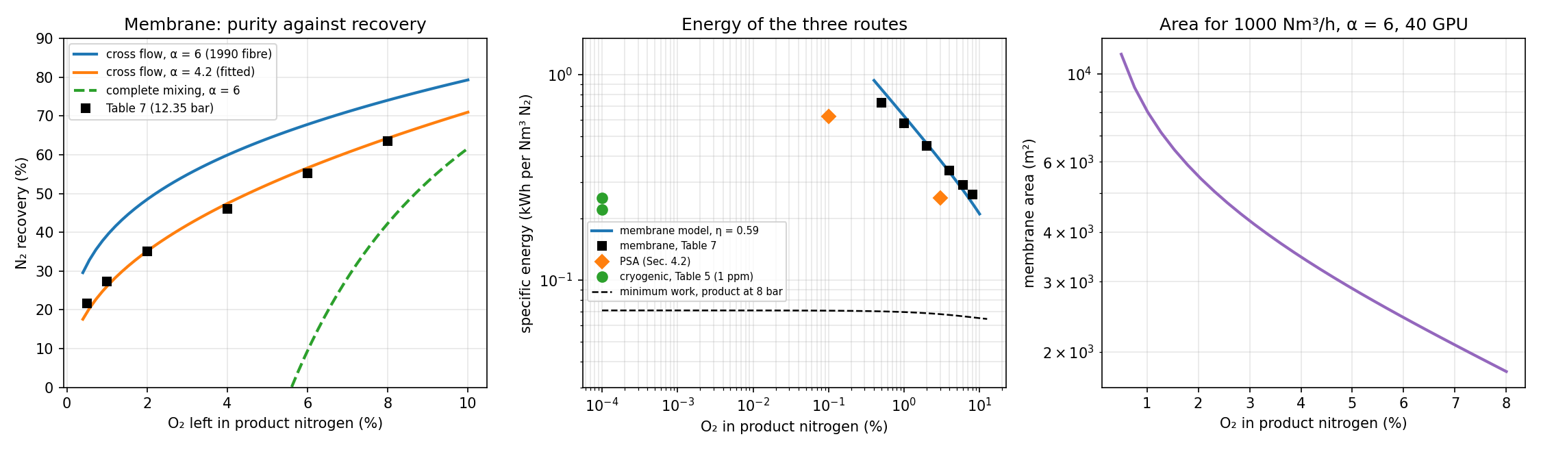
**Figure 3.** Left: nitrogen recovery against residual oxygen for cross flow and complete mixing, with the performance data of Ullmann’s Table 7 (air at 12.35 bar). Middle: specific energy of the three routes against product purity, with the thermodynamic minimum for a product at 8 bar. Right: membrane area for 1000 Nm³/h of product with the fibres of Ullmann’s 1990 example.

Häussinger et al. give the performance of a membrane generator fed with air at 12.35 bar: 21.7 % of the nitrogen is recovered at 0.5 % O₂ and 63.6 % at 8 % O₂ (Häussinger et al., 2000a, Table 7). The cross-flow model reproduces these data within 1.4 points of recovery with an effective selectivity α = 4.2, the value of poly(4-methyl-1-pentene) in their Table 6 (Häussinger et al., 2000a, Table 6). The fibre they describe as the state of the art in 1990, with α = 6, would recover 39 % instead of 27 % at 1 % O₂ (Häussinger et al., 2000a, Sec. 4.3). Complete mixing is much worse: with α = 6 its retentate cannot go below 4.2 % O₂ even at zero recovery, because the permeate can never be richer in oxygen than αx/[1 + (α − 1)x] of the retentate (Strathmann, 2005, Eq. 4.20). Flow pattern matters as much as the membrane.

With the 1990 fibre (2 Barrer of oxygen through a 50 nm skin, 40 GPU) 1000 Nm³/h of nitrogen with 1 % O₂ needs about 8100 m² of membrane, some 2.6 million fibres of 0.5 mm outer diameter and 2 m length (Häussinger et al., 2000a, Sec. 4.3).

The energy of all three routes is almost entirely the work of the air compressor. It is compared with the isothermal compression work, and with the ideal work of the separation, the minimum any process needs, for ideal gases with T₀ = 298 K (Smith et al., 2018, Eqs. 5.21, 5.23 and 10.26):

$$\begin{gathered}w = \frac{R\,T_0\,\ln(p_f/p_0)}{\eta_T}\ \text{per mol of air} \\[6pt] W_{ideal} = \Delta H - T_0\,\Delta S, \qquad S^{ig} = \sum_i y_i S_i^{ig} - R\sum_i y_i \ln y_i, \qquad \eta_t = \frac{W_{ideal}}{W_s}\end{gathered}$$Eq. 7 — compression work and ideal work

Route and data	Purity	Energy, kWh/Nm³ N₂	Implied η_T
Single column, 8 bar (Häussinger et al., 2000a, Table 5)	1 ppm O₂	0.25	0.52 (with the 64 % recovery of Solution 2)
Double column, N₂ compressed to 8 bar (Häussinger et al., 2000a, Table 5)	1 ppm O₂	0.22	—
PSA, carbon molecular sieve (Häussinger et al., 2000a, Sec. 4.2)	1000 ppm / 3 %	0.63 / 0.25	—
Membrane, 12.35 bar (Häussinger et al., 2000a, Table 7)	0.5 % / 8 %	0.73 / 0.26	0.54–0.61
Ideal work, product at 8 bar	1 ppm O₂	0.071–0.075	—

Two conclusions follow. First, the tables are internally consistent: with the recoveries of the models, the cryogenic and the membrane energies both correspond to an overall isothermal efficiency of the compressor and its drive of about 0.5–0.6. Second, the ideal work is only 0.07 kWh/Nm³, and nine tenths of it is the compression of the product to 8 bar, not the separation. The cryogenic single column works at a second-law efficiency of about 30 %. Membranes and PSA lose most at high purity, where their recovery collapses and most of the compressed air is thrown away. This is the thermodynamic content of Ullmann's map of cost-effective regions (Häussinger et al., 2000a, Fig. 3).

air_membrane.pyDownload

"""
Air separation — membrane nitrogen generator and the energy of the three routes
bdrworks.org · Handbook · Air separation, worked model 3

Compressed air flows along hollow fibres; O2 permeates faster than N2 and the N2-rich
retentate is the product. Binary O2/N2 model (argon counted with nitrogen), permeate at
1 bar. Local permeate composition (Weller–Steiner):
    y/(1-y) = alpha (x - phi y) / ((1 - x) - phi (1 - y)),     phi = p_permeate/p_feed
Complete mixing: the whole feed side is at the retentate composition.
Cross flow: each element's permeate leaves without mixing; along the fibre
    d(n)/d(x) = n/(y - x),     dA = -dn / J,   J = Q_O2 (p_f x - p_p y) + Q_N2 (p_f (1-x) - p_p (1-y))
The energy is the air compression, w = R T0 ln(p_f/p0) / eta_T per mol of air, and the
thermodynamic minimum follows from the ideal work of separating ideal gases.

Run:  python air_membrane.py      (needs numpy, scipy, matplotlib)
"""
import numpy as np
from scipy.integrate import solve_ivp
from scipy.optimize import brentq, minimize_scalar
import matplotlib.pyplot as plt

RG, T0, VN = 8.314462618, 298.15, 0.022414        # J/(mol K), K, m3(STP)/mol
XF = 0.2095                                        # O2 in dry air
GPU = 3.3464e-10                                   # mol/(m2 s Pa) per GPU

# Table 7 of Häussinger et al. (Ullmann, Nitrogen): air at 12.35 bar
TABLE7 = [(0.005, 21.7, 0.73), (0.01, 27.3, 0.58), (0.02, 35.0, 0.45), (0.04, 46.1, 0.34), (0.06, 55.2, 0.29), (0.08, 63.6, 0.26)]
PF, PP = 12.35, 1.013


def y_local(x, a, phi):
    """Root in (0, 1) of phi(1 - a) y^2 + [1 + (a - 1)(x + phi)] y - a x = 0."""
    A, B, C = phi*(1 - a), 1 + (a - 1)*(x + phi), -a*x
    return -2*C/(B + np.sqrt(B*B - 4*A*C))


def cross_flow(a, phi, xr, xf=XF):
    """Retentate flow per mol of feed when the O2 fraction is brought from xf to xr."""
    sol = solve_ivp(lambda x, n: [n[0]/(y_local(x, a, phi) - x)], (xf, xr), [1.0], rtol=1e-10, atol=1e-12)
    return sol.y[0, -1]


def complete_mixing(a, phi, xr, xf=XF):
    y = y_local(xr, a, phi)
    theta = (xf - xr)/(y - xr)                    # stage cut
    return 1.0 - theta if 0 <= theta <= 1 else np.nan


def recovery(nr, xr, xf=XF):
    return nr*(1 - xr)/(1 - xf)


def cross_flow_area(a, QO2_gpu, pf, pp, xr, xf=XF):
    """Membrane area (m2) per mol/s of feed air, cross flow."""
    QO2, QN2 = QO2_gpu*GPU, QO2_gpu*GPU/a
    phi = pp/pf
    def rhs(x, u):
        n = u[0]; y = y_local(x, a, phi)
        dn = n/(y - x)
        J = QO2*(pf*1e5*x - pp*1e5*y) + QN2*(pf*1e5*(1 - x) - pp*1e5*(1 - y))
        return [dn, -dn/J]
    sol = solve_ivp(rhs, (xf, xr), [1.0, 0.0], rtol=1e-9, atol=1e-12)
    return sol.y[1, -1]


def w_min(yp, Pp, R, P0=1.0, z=(XF, 1 - XF)):
    """Ideal work (J per mol of product) to make product (O2 fraction yp) at Pp from air at P0,
    with nitrogen recovery R and the reject at P0 (ideal gases at T0)."""
    z = np.array(z); npr = R*z[1]/(1 - yp); nw = 1 - npr
    yw = (z[0] - npr*yp)/nw
    s = lambda y, P: sum(v*np.log(v*P/P0) for v in y if v > 0)
    return RG*T0*(npr*s([yp, 1 - yp], Pp) + nw*s([yw, 1 - yw], P0) - s(z, P0))/npr


def kwh_per_nm3(J_per_mol):
    return J_per_mol/VN/3.6e6


if __name__ == "__main__":
    phi = PP/PF
    fit = minimize_scalar(lambda a: sum((100*recovery(cross_flow(a, phi, xr), xr) - rec)**2 for xr, rec, _ in TABLE7),
                          bounds=(2.5, 8.0), method="bounded")
    a_fit = fit.x
    print(f"cross flow fitted to Table 7: alpha = {a_fit:.2f} (rms {np.sqrt(fit.fun/len(TABLE7)):.1f} points of recovery)")
    print("O2 %   Table 7   cross(fit)   cross(alpha 6)   complete(alpha 6)")
    for xr, rec, E in TABLE7:
        print(f"{100*xr:4.1f}   {rec:5.1f}    {100*recovery(cross_flow(a_fit, phi, xr), xr):6.1f}      "
              f"{100*recovery(cross_flow(6.0, phi, xr), xr):6.1f}        {100*recovery(complete_mixing(6.0, phi, xr), xr):6.1f}")
    x_lim = XF/(6.0 - 5.0*XF)
    print(f"complete mixing, alpha 6, phi -> 0: the retentate cannot fall below {100*x_lim:.2f} % O2")

    # energy: isothermal compression implied by the tables
    w_air = RG*T0*np.log(PF/1.013)
    etas = []
    for xr, rec, E in TABLE7:
        air_per_prod = (1 - xr)/(rec/100*(1 - XF))
        eta = kwh_per_nm3(w_air*air_per_prod)/E; etas.append(eta)
    print(f"Table 7 energies imply an isothermal compression efficiency of {min(etas):.2f}–{max(etas):.2f}")
    # cryogenic single column (Table 5): 0.25 kWh/m3 N2 at 8 bar; recovery from air_column.py (40 stages, 1 ppm): 64.0 %
    rec_col = 0.640; w_col = RG*T0*np.log(8.5/1.013)/(rec_col*(1 - XF))
    print(f"single column, 64 % recovery, air to 8.5 bar: isothermal work {kwh_per_nm3(w_col):.3f} kWh/Nm3 -> "
          f"Table 5 (0.25) implies eta = {kwh_per_nm3(w_col)/0.25:.2f}")
    for yp, Pp, R, lab in [(1e-6, 8.0, 0.64, "single column, 1 ppm, 8 bar, 64 %"), (1e-6, 8.0, 1e-6, "same, vanishing recovery"),
                           (0.01, 11.35, 0.273, "membrane, 1 % O2, 27 %"), (0.01, 11.35, 1e-6, "membrane product, vanishing recovery")]:
        print(f"minimum work, {lab}: {kwh_per_nm3(w_min(yp, Pp, R)):.4f} kWh/Nm3")
    A = cross_flow_area(6.0, 40.0, PF, PP, 0.01)
    nr = cross_flow(6.0, phi, 0.01); prod = 1000/3600/VN                   # 1000 Nm3/h of product, mol/s
    area = A*prod/nr
    print(f"alpha 6, 40 GPU O2 fibres (2 Barrer, 50 nm skin): {area:.0f} m2 for 1000 Nm3/h at 1 % O2 "
          f"= {area/(np.pi*500e-6*2.0)/1e6:.2f} million fibres of 0.5 mm x 2 m")

    fig, ax = plt.subplots(1, 3, figsize=(15, 4.4))
    xs = np.linspace(0.004, 0.10, 60)
    ax[0].plot(100*xs, [100*recovery(cross_flow(6.0, phi, x), x) for x in xs], lw=2, label="cross flow, α = 6 (1990 fibre)")
    ax[0].plot(100*xs, [100*recovery(cross_flow(a_fit, phi, x), x) for x in xs], lw=2, label=f"cross flow, α = {a_fit:.1f} (fitted)")
    rc = [100*recovery(complete_mixing(6.0, phi, x), x) for x in xs]
    ax[0].plot(100*xs, [r if r > 0 else np.nan for r in rc], lw=2, ls="--", label="complete mixing, α = 6")
    ax[0].plot([100*t[0] for t in TABLE7], [t[1] for t in TABLE7], "ks", label="Table 7 (12.35 bar)")
    ax[0].set(xlabel="O₂ left in product nitrogen (%)", ylabel="N₂ recovery (%)", title="Membrane: purity against recovery", ylim=(0, 90))
    ax[0].legend(fontsize=8); ax[0].grid(alpha=0.3)

    eta = float(np.mean(etas))
    ax[1].loglog(100*xs, [kwh_per_nm3(w_air*(1 - x)/(recovery(cross_flow(a_fit, phi, x), x)*(1 - XF)))/eta for x in xs], lw=2,
                 label=f"membrane model, η = {eta:.2f}")
    ax[1].loglog([100*t[0] for t in TABLE7], [t[2] for t in TABLE7], "ks", label="membrane, Table 7")
    ax[1].loglog([3.0, 0.1], [0.2*1.2505, 0.5*1.2505], "D", color="tab:orange", ms=7, label="PSA (Sec. 4.2)")
    ax[1].loglog([1e-4, 1e-4], [0.25, 0.22], "o", color="tab:green", ms=7, label="cryogenic, Table 5 (1 ppm)")
    yps = np.logspace(-6, -0.9, 50)
    ax[1].loglog(100*yps, [kwh_per_nm3(w_min(y, 8.0, 1e-6)) for y in yps], "k--", lw=1.2, label="minimum work, product at 8 bar")
    ax[1].set(xlabel="O₂ in product nitrogen (%)", ylabel="specific energy (kWh per Nm³ N₂)", title="Energy of the three routes", ylim=(0.03, 1.5))
    ax[1].legend(fontsize=7, loc="center left", bbox_to_anchor=(0.0, 0.36)); ax[1].grid(alpha=0.3, which="both")

    xa = np.linspace(0.005, 0.08, 30)
    areas = [cross_flow_area(6.0, 40.0, PF, PP, x)*prod/cross_flow(6.0, phi, x) for x in xa]
    ax[2].semilogy(100*xa, areas, lw=2, color="tab:purple")
    ax[2].set(xlabel="O₂ in product nitrogen (%)", ylabel="membrane area (m²)", title="Area for 1000 Nm³/h, α = 6, 40 GPU")
    ax[2].grid(alpha=0.3, which="both")
    fig.tight_layout(); fig.savefig("air_membrane.png", dpi=150)
    plt.show()

air_membrane.mDownload

function air_membrane()
% Air separation - membrane nitrogen generator (hollow fibres) and the energy of the three routes
% bdrworks.org - Handbook - Air separation, worked model 3
%   binary O2/N2, local permeate from phi(1-a) y^2 + [1 + (a-1)(x+phi)] y - a x = 0
%   complete mixing and cross flow (dn/dx = n/(y - x)); energy w = R T0 ln(pf/p0)/eta per mol air
% Save as air_membrane.m and run:  air_membrane      (MATLAB or GNU Octave)

xf = 0.2095;  PF = 12.35;  PP = 1.013;  phi = PP/PF;  R = 8.314462618;  T0 = 298.15;
tab = [0.005 21.7 0.73; 0.01 27.3 0.58; 0.02 35.0 0.45; 0.04 46.1 0.34; 0.06 55.2 0.29; 0.08 63.6 0.26];
err = @(a) sum((arrayfun(@(k) 100*recov(crossflow(a, phi, tab(k,1), xf), tab(k,1), xf), 1:6)' - tab(:,2)).^2);
afit = fminbnd(err, 2.5, 8);
fprintf('cross flow fitted to Table 7: alpha = %.2f (rms %.1f points)\n', afit, sqrt(err(afit)/6));
for k = 1:6
    x = tab(k,1);
    fprintf('%4.1f %% O2: Table 7 %5.1f, cross(fit) %5.1f, cross(alpha 6) %5.1f, complete(alpha 6) %6.1f\n', 100*x, tab(k,2), ...
            100*recov(crossflow(afit, phi, x, xf), x, xf), 100*recov(crossflow(6, phi, x, xf), x, xf), 100*recov(complete(6, phi, x, xf), x, xf));
end
fprintf('complete mixing, alpha 6, phi -> 0: the retentate cannot fall below %.2f %% O2\n', 100*xf/(6 - 5*xf));
wair = R*T0*log(PF/PP);  eta = zeros(6,1);
for k = 1:6
    eta(k) = kwh(wair*(1 - tab(k,1))/(tab(k,2)/100*(1 - xf)))/tab(k,3);
end
fprintf('Table 7 energies imply an isothermal compression efficiency of %.2f-%.2f\n', min(eta), max(eta));
wcol = R*T0*log(8.5/1.013)/(0.640*(1 - xf));
fprintf('single column, 64 %% recovery: isothermal work %.3f kWh/Nm3 -> Table 5 (0.25) implies eta = %.2f\n', kwh(wcol), kwh(wcol)/0.25);
fprintf('minimum work, 1 ppm N2 at 8 bar, 64 %% recovery: %.4f kWh/Nm3\n', kwh(wmin(1e-6, 8, 0.64, xf)));
fprintf('minimum work, 1 %% O2 at 11.35 bar, 27 %% recovery: %.4f kWh/Nm3\n', kwh(wmin(0.01, 11.35, 0.273, xf)));
prod = 1000/3600/0.022414;
A = area(6, 40, PF, PP, 0.01, xf)*prod/crossflow(6, phi, 0.01, xf);
fprintf('alpha 6, 40 GPU fibres: %.0f m2 for 1000 Nm3/h at 1 %% O2\n', A);

xs = linspace(0.004, 0.10, 40);
figure('Position', [60 100 1300 380]);
subplot(1,3,1);
plot(100*xs, arrayfun(@(x) 100*recov(crossflow(6, phi, x, xf), x, xf), xs), ...
     100*xs, arrayfun(@(x) 100*recov(crossflow(afit, phi, x, xf), x, xf), xs), 'LineWidth', 2); hold on;
plot(100*tab(:,1), tab(:,2), 'ks');
xlabel('O_2 in product (%)'); ylabel('N_2 recovery (%)'); title('Membrane: purity against recovery');
legend('cross flow, \alpha = 6', 'cross flow, fitted \alpha', 'Table 7'); grid on;
subplot(1,3,2);
loglog(100*tab(:,1), tab(:,3), 'ks', [3 0.1], [0.2 0.5]*1.2505, 'd', [1e-4 1e-4], [0.25 0.22], 'o'); hold on;
yps = logspace(-6, -0.9, 30);
loglog(100*yps, arrayfun(@(y) kwh(wmin(y, 8, 1e-6, xf)), yps), 'k--');
xlabel('O_2 in product (%)'); ylabel('kWh per Nm^3 N_2'); title('Energy of the three routes');
legend('membrane (Table 7)', 'PSA', 'cryogenic (Table 5)', 'minimum work'); grid on;
subplot(1,3,3);
xa = linspace(0.005, 0.08, 20);
semilogy(100*xa, arrayfun(@(x) area(6, 40, PF, PP, x, xf)*prod/crossflow(6, phi, x, xf), xa), 'LineWidth', 2);
xlabel('O_2 in product (%)'); ylabel('membrane area (m^2)'); title('Area for 1000 Nm^3/h'); grid on;
end

function y = ylocal(x, a, phi)
A = phi*(1 - a);  B = 1 + (a - 1)*(x + phi);  C = -a*x;
y = -2*C/(B + sqrt(B^2 - 4*A*C));
end

function nr = crossflow(a, phi, xr, xf)
opts = odeset('RelTol', 1e-10, 'AbsTol', 1e-12);
[~, n] = ode45(@(x, n) n/(ylocal(x, a, phi) - x), [xf xr], 1, opts);
nr = n(end);
end

function nr = complete(a, phi, xr, xf)
y = ylocal(xr, a, phi);  th = (xf - xr)/(y - xr);
if th >= 0 && th <= 1, nr = 1 - th; else, nr = NaN; end
end

function r = recov(nr, xr, xf),  r = nr*(1 - xr)/(1 - xf);  end
function e = kwh(J),  e = J/0.022414/3.6e6;  end

function A = area(a, QO2gpu, pf, pp, xr, xf)
% membrane area per mol/s of feed air, cross flow
GPU = 3.3464e-10;  QO2 = QO2gpu*GPU;  QN2 = QO2/a;  phi = pp/pf;
f = @(x, u) [u(1)/(ylocal(x, a, phi) - x); ...
             -(u(1)/(ylocal(x, a, phi) - x))/(QO2*(pf*1e5*x - pp*1e5*ylocal(x, a, phi)) + QN2*(pf*1e5*(1 - x) - pp*1e5*(1 - ylocal(x, a, phi))))];
opts = odeset('RelTol', 1e-9, 'AbsTol', 1e-12);
[~, u] = ode45(f, [xf xr], [1; 0], opts);
A = u(end, 2);
end

function w = wmin(yp, Pp, Rn, xf)
% ideal work, J per mol of product (O2 fraction yp at Pp bar), N2 recovery Rn, reject at 1 bar, T0 = 298.15 K
RT = 8.314462618*298.15;  np = Rn*(1 - xf)/(1 - yp);  nw = 1 - np;  yw = (xf - np*yp)/nw;
s = @(y, P) sum(y(y > 0).*log(y(y > 0)*P));
w = RT*(np*s([yp 1-yp], Pp) + nw*s([yw 1-yw], 1) - s([xf 1-xf], 1))/np;
end

7Model and plant

Quantity	Model	Literature
N₂ vapour pressure, 80 / 100 / 120 K	1.371 / 7.806 / 25.11 bar	1.367 / 7.777 / 25.13 bar (Häussinger et al., 2000a, Table 1)
N₂ latent heat, 80 / 100 K	5.52 / 4.48 kJ/mol	5.47 / 4.50 kJ/mol (Häussinger et al., 2000a, Table 1)
Air condenses at 1 / 6 bar	82.1 / 101.4 K	81.5 / 101 K (Häussinger et al., 2000a, Sec. 4.1)
HP / LP pressures of a double column	5.3 / 1.3 bar for ΔT = 2 K	ΔT of about 2 K (Häussinger et al., 2000a, Fig. 4)
Single-column product purity	1 ppm O₂ at 30–40 stages	about 1 ppm O₂, with argon (Häussinger et al., 2000a, Sec. 4.1)
Membrane recovery, 0.5–8 % O₂	19–64 % (α = 4.2)	21.7–63.6 % (Häussinger et al., 2000a, Table 7)
Oxygen from air (20 % O₂ as in Strathmann), silicone membrane (α = 2), φ → 0	33.3 %	about 33 % (Strathmann, 2005, Fig. 26)

8Try it

The three models run below in JavaScript. The column is solved with the same bubble-point method as the Python and MATLAB codes, and the membrane with a fixed-step Runge–Kutta integration.

Pressure (bar)

LP column pressure (bar)

Condenser ΔT (K)

Column pressure (bar)

Equilibrium stages

Product D (mol per mol air)

Selectivity α O₂/N₂

Feed pressure (bar)

Permeate pressure (bar)

O₂ in product (%)

O₂ permeance (GPU)

Product (Nm³/h)

Compressor η_T

9Going further

Add the LP column of a double column: feed the bottom liquid of an HP column at 5.3 bar (Solution 2 run at that pressure) to its middle and the HP top liquid as reflux, and find the oxygen purity against the number of stages (Häussinger et al., 2000a, Fig. 6).
Replace constant molar overflow with enthalpy balances (the sum-rates method) and close the heat balance of the condenser (Walas, 1990, Sec. 13.10).
Draw off the liquid at the argon maximum of Solution 2 as the feed of a side column and estimate how much argon it could recover.
Integrate the counter-current flow pattern of the membrane as a boundary-value problem and compare it with cross flow (Strathmann, 2005, Fig. 28; Finlayson et al., 2006, Sec. 7.2).
Estimate the refrigeration balance of the cold box: the 415 kJ/kg to cool and liquefy air against the heat recovered from the products and the work of the expansion turbine (Häussinger et al., 2000a, Sec. 4.1).

10References

Brent, R. P. (1973). Algorithms for Minimization without Derivatives. Prentice-Hall, Englewood Cliffs, NJ.
Dormand, J. R., & Prince, P. J. (1980). A family of embedded Runge–Kutta formulae. J. Comput. Appl. Math., 6(1), 19–26.
Finlayson, B. A., Biegler, L. T., & Grossmann, I. E. (2006). Mathematics in chemical engineering. In Ullmann's Encyclopedia of Industrial Chemistry. Wiley-VCH, Weinheim. doi:10.1002/14356007.b01_01.pub2
Häussinger, P., Glatthaar, R., Rhode, W., Kick, H., Benkmann, C., Weber, J., Wunschel, H.-J., Stenke, V., Leicht, E., & Stenger, H. (2000b). Noble gases. In Ullmann's Encyclopedia of Industrial Chemistry. Wiley-VCH, Weinheim. doi:10.1002/14356007.a17_485
Häussinger, P., Leitgeb, P., & Schmücker, B. (2000a). Nitrogen. In Ullmann's Encyclopedia of Industrial Chemistry. Wiley-VCH, Weinheim. doi:10.1002/14356007.a17_457
Lee, B. I., & Kesler, M. G. (1975). A generalized thermodynamic correlation based on three-parameter corresponding states. AIChE J., 21(3), 510–527.
NOAA, NASA, & USAF (1976). U.S. Standard Atmosphere, 1976 (NOAA-S/T 76-1562). U.S. Government Printing Office, Washington, DC.
Peng, D.-Y., & Robinson, D. B. (1976). A new two-constant equation of state. Ind. Eng. Chem. Fundam., 15(1), 59–64.
Smith, J. M., Van Ness, H. C., Abbott, M. M., & Swihart, M. T. (2018). Introduction to Chemical Engineering Thermodynamics (8th ed.). McGraw-Hill Education, New York.
Strathmann, H. (2005). Membranes and membrane separation processes. In Ullmann's Encyclopedia of Industrial Chemistry. Wiley-VCH, Weinheim. doi:10.1002/14356007.a16_187.pub2
Walas, S. M. (1990). Chemical Process Equipment: Selection and Design. Butterworth-Heinemann, Boston.
Wang, J. C., & Henke, G. E. (1966). Tridiagonal matrix for distillation. Hydrocarbon Process., 45(8), 155–163.
Weller, S., & Steiner, W. A. (1950). Engineering aspects of separation of gases: fractional permeation through membranes. Chem. Eng. Prog., 46, 585–590.

The plant cases follow the descriptions and tables in Ullmann's Encyclopedia; the number of stages, the temperature approach and the compressor efficiency are round-number assumptions for teaching, not data from a specific plant.

Air separationmodeling.