1The problem
Methanol is made from synthesis gas — H₂, CO and CO₂ — over a copper catalyst at 50–100 bar and 200–300 °C, the conditions of the low-pressure process (Fiedler et al., 2000, Secs. 5 and 5.2). The chemistry resembles ammonia synthesis: reversible, exothermic, fewer moles on the product side, and limited by equilibrium to a few percent of methanol per pass. Two things make it harder. There are two independent reactions instead of one, and the copper catalyst loses activity by sintering when it is overheated, so temperature control is even more critical than for iron ammonia catalyst (Fiedler et al., 2000, Sec. 4.2.4).
The three solutions follow the two main reactor types of the process. The ICI reactor is a single adiabatic catalyst bed in which the reaction is quenched by cold gas added at several points. The Lurgi reactor is a tubular reactor cooled by boiling water. Between them these two designs accounted for about 90 % of world production when the Ullmann article was written (Fiedler et al., 2000, Sec. 5.3). Finally, no converter works alone: the synthesis loop, with recycle and purge, sets the real production.
2Process and catalyst
Modern plants run the low-pressure process introduced by ICI in 1966, which replaced the old zinc oxide–chromium oxide catalyst used at 25–35 MPa and 300–450 °C; the last high-pressure plant closed in the mid-1980s (Fiedler et al., 2000, Secs. 4.2.1 and 4.2.2). The catalyst is copper on zinc oxide with an alumina promoter, usually pressed into cylindrical tablets of 4–6 mm, with a selectivity above 99 % and a useful life of 2–5 years (Fiedler et al., 2000, Secs. 4.1.3, 4.2.3 and 4.2.4). Isotope experiments showed that on this catalyst methanol is formed mainly from CO₂, not CO (Chinchen et al., 1987; Fiedler et al., 2000, Sec. 4.1.2). CO takes part through the water-gas shift, which turns it into CO₂ and at the same time consumes the water produced by methanol synthesis. The network is therefore best written as CO₂ hydrogenation plus the (reverse) water-gas shift:
The make-up gas is characterised by the stoichiometric number, which should be at least 2 (Fiedler et al., 2000, Sec. 5.1):
SN = 2 provides exactly the hydrogen needed for both carbon oxides. Gas from steam reforming of natural gas is hydrogen-rich, well above SN = 2. The excess hydrogen accumulates in the loop and leaves with the purge, which is normally burnt in the reformer furnace (Fiedler et al., 2000, Secs. 5.1 and 5.2). That is why the make-up gas in Solution 3 has SN = 2.56 and why the purge matters so much.
3Equilibrium
With two independent reactions the equilibrium is found from two extents of reaction, ξ₁ and ξ₂. Every flow is ni = ni,0 + νi1ξ₁ + νi2ξ₂, and the two equilibrium conditions are solved together, with the equilibrium constants of Graaf et al. (Graaf et al., 1986; Smith et al., 2018, Sec. 14.9):
The two conditions are solved in logarithmic form with a Newton-type solver. As in the kinetic model they were fitted with, the gas is treated as ideal. At these pressures that slightly underestimates methanol formation, a known limitation that is absorbed into the kinetic constants. Ullmann notes that published formulations of the equilibrium constants differ widely, and that fugacity coefficients from an equation of state such as Soave–Redlich–Kwong should be used for accurate equilibrium work (Fiedler et al., 2000, Sec. 4.1.1).
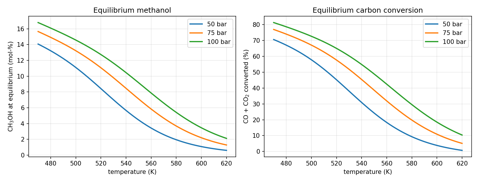
At 523 K the equilibrium methanol content of this gas is 8.0 % at 50 bar, 10.7 % at 75 bar and 12.4 % at 100 bar. It falls by roughly half for every 40 K rise in temperature. Every reactor below is judged against this curve.
The supporting script meoh_equilibrium.py reproduces Figure 1.
4Kinetics
The kinetic model of Vanden Bussche and Froment is the most widely used for commercial Cu/ZnO/Al₂O₃ catalyst. It is derived from a surface mechanism in which CO₂ adsorbs and is hydrogenated step by step through formate species, and the water-gas shift proceeds by a redox mechanism on copper. Both rates share one adsorption term β (Vanden Bussche & Froment, 1996):
The rate constants have the form k = A exp(B/RT) with:
| Constant | A | B (J/mol) | Units |
|---|---|---|---|
| k₁ | 1.07 | 36 696 | mol/(kg s bar²) |
| k₂ | 3 453.38 | 0 | — |
| k₃ | 0.499 | 17 197 | bar⁻⁰·⁵ |
| k₄ | 6.62 × 10⁻¹¹ | 124 119 | bar⁻¹ |
| k₅ | 1.22 × 10¹⁰ | −94 765 | mol/(kg s bar) |
The term k₂pH₂O/pH₂ in β stands for water blocking the active sites. Water is the reason methanol synthesis slows down so strongly along the bed, and the reason that removing CO₂ entirely would not help: the catalyst needs a few percent of CO₂, but too much produces water that inhibits it (Vanden Bussche & Froment, 1996; Fiedler et al., 2000, Sec. 4.1.2).
5Reactor model
The model assumes one-dimensional pseudo-homogeneous plug flow, which predicts the radially averaged temperature well as long as radial gradients stay mild (Hlavacek et al., 2000, Sec. 4.3), no pressure drop, no intraparticle limitations beyond what is lumped into the rate constants, and ideal-gas heat capacities (Reid, Prausnitz and Poling polynomials) with heats of reaction from the enthalpies of formation (Poling et al., 2001, App. A; Froment et al., 2011, Ch. 11). Seven species (CO, CO₂, H₂, CH₃OH, H₂O, CH₄, N₂) and two reactions give:
The adiabatic beds of Solution 1 use the same balances with catalyst mass as the coordinate and U = 0. The tube-cooled reactor of Solution 2 models one representative tube (D = 40 mm, L = 7 m, ρb = 1 140 kg/m³, U = 250 W/m²K) and multiplies it by 5 000 tubes. Both reactors therefore hold the same 50 t of catalyst.
6Solution 1 · Quench converter
In the ICI converter the catalyst is one large adiabatic bed, and cold gas is injected at several levels through distributors, so the axial temperature profile has a sawtooth shape (Fiedler et al., 2000, Sec. 5.3). The model treats the catalyst between two injection levels as an adiabatic bed. Only part of the feed is preheated and sent to the top; the rest stays cold and is injected at the quench points. The quench flow before each bed follows from an enthalpy balance of the mixing point:
All quench streams plus the bed-1 flow must add up to the whole feed. That gives one equation for the unknown fraction to bed 1, solved with a bracketing root finder (brentq / fzero) around the full bed sequence (Brent, 1973).
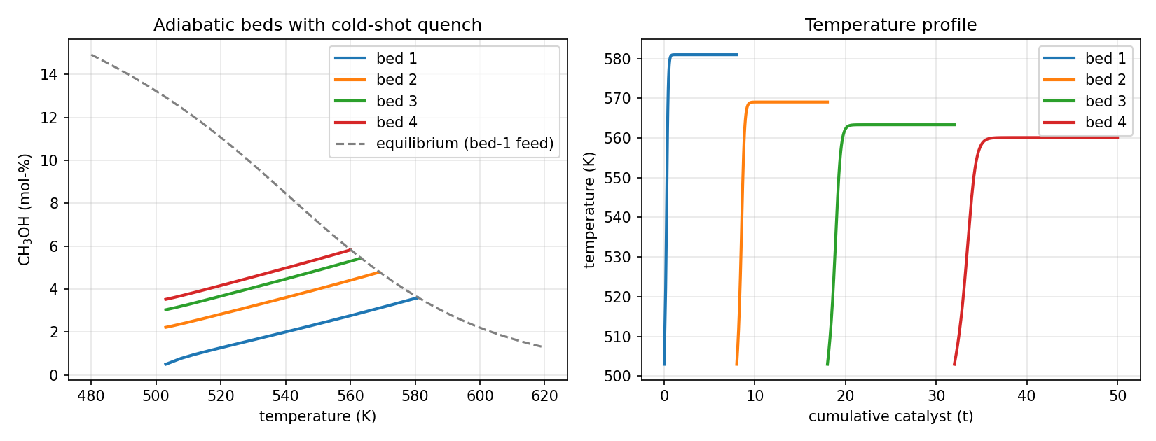
| Bed | Catalyst | T in → out | CH₃OH out | Equilibrium at T out |
|---|---|---|---|---|
| 1 (22 % of feed) | 8 t | 503 → 581 K | 3.61 % | 3.61 % |
| 2 | 10 t | 503 → 569 K | 4.79 % | 4.79 % |
| 3 | 14 t | 503 → 563 K | 5.44 % | 5.44 % |
| 4 | 18 t | 503 → 560 K | 5.83 % | 5.83 % |
The converter makes 477 kmol/h, about 370 t/d. Two weaknesses stand out:
- Every bed runs into equilibrium within the first metre or so. Most of the catalyst sits at a high temperature where the equilibrium no longer allows more methanol.
- Quenching dilutes the product with unreacted gas instead of removing heat. The final mixture has only 5.8 % methanol, and the first bed reaches 581 K, above the 200–300 °C range of industrial reactors, where copper sintering accelerates (Fiedler et al., 2000, Secs. 4.2.4 and 5.2).
The quench design survives because it is simple and scales to very large single converters. Its temperature problem is handled in practice with a leaner, more diluted loop gas.
"""
Methanol synthesis — adiabatic multi-bed quench converter (ICI type)
bdrworks.org · Handbook · Methanol, worked model 1

Four adiabatic catalyst beds. Only part of the feed is preheated and sent to bed 1;
the rest stays cold (quench gas) and is injected between the beds so that every
bed starts at the same inlet temperature.
    dF_i/dW = sum_j nu_ij r_j               (W = catalyst mass, kg)
    (sum F_i cp_i) dT/dW = sum_j (-dH_j) r_j
The quench flow before each bed follows from an enthalpy balance of the mixing
point, and the split of the feed is found so that all of it is used.

Run:  python meoh_quench.py      (needs numpy, scipy, matplotlib)
"""
import numpy as np
from scipy.integrate import solve_ivp
from scipy.optimize import brentq
import matplotlib.pyplot as plt

# ---------------------------------------------------------------- data
SPECIES = ["CO", "CO2", "H2", "CH3OH", "H2O", "CH4", "N2"]
#                 CO   CO2   H2  MeOH  H2O  CH4  N2
NU = np.array([[0.0, -1.0, -3.0, 1.0, 1.0, 0.0, 0.0],     # 1: CO2 + 3H2 <=> CH3OH + H2O
               [1.0, -1.0, -1.0, 0.0, 1.0, 0.0, 0.0]])    # 2: CO2 + H2  <=> CO + H2O (RWGS)
RG = 8.314                                                 # J/(mol K)

# ideal-gas cp = A + B T + C T^2 + D T^3, J/(mol K)  (Reid, Prausnitz & Poling)
CP = np.array([[30.87, -1.285e-2, 2.789e-5, -1.272e-8],   # CO
               [19.80, 7.344e-2, -5.602e-5, 1.715e-8],    # CO2
               [27.14, 9.274e-3, -1.381e-5, 7.645e-9],    # H2
               [21.15, 7.092e-2, 2.587e-5, -2.852e-8],    # CH3OH
               [32.24, 1.924e-3, 1.055e-5, -3.596e-9],    # H2O
               [19.25, 5.213e-2, 1.197e-5, -1.132e-8],    # CH4
               [31.15, -1.357e-2, 2.680e-5, -1.168e-8]])  # N2
HF = np.array([-110.53, -393.51, 0.0, -200.94, -241.83, -74.87, 0.0]) * 1e3   # J/mol, 298.15 K


def cp(T):
    """Heat capacities of all species, J/(mol K)."""
    return CP @ np.array([1.0, T, T**2, T**3])


def h(T):
    """Molar enthalpies H_f(298) + integral of cp, J/mol."""
    T0 = 298.15
    dT = np.array([T - T0, (T**2 - T0**2) / 2, (T**3 - T0**3) / 3, (T**4 - T0**4) / 4])
    return HF + CP @ dT


def dH_rxn(T):
    """Heats of reaction 1 and 2, J/mol."""
    return NU @ h(T)


def K_eq(T):
    """Equilibrium constants (Graaf et al.), partial pressures in bar.
    K1 for CO2 + 3H2 = CH3OH + H2O (bar^-2);  K3 for CO + H2O = CO2 + H2 (-)."""
    K1 = 10.0 ** (3066.0 / T - 10.592)
    K3 = 10.0 ** (2073.0 / T - 2.029)
    return K1, K3


def rates(T, p):
    """Vanden Bussche & Froment (1996) rates, mol/(kg_cat s); p = partial pressures in bar."""
    pCO, pCO2, pH2, pM, pW = [max(x, 1e-10) for x in p[:5]]
    k = lambda A, B: A * np.exp(B / (RG * T))
    k1, k2, k3, k4, k5 = k(1.07, 36696), k(3453.38, 0), k(0.499, 17197), k(6.62e-11, 124119), k(1.22e10, -94765)
    K1, K3 = K_eq(T)
    den = 1.0 + k2 * pW / pH2 + k3 * np.sqrt(pH2) + k4 * pW
    r1 = k1 * pCO2 * pH2 * (1.0 - pW * pM / (K1 * pH2**3 * pCO2)) / den**3
    r2 = k5 * pCO2 * (1.0 - K3 * pW * pCO / (pCO2 * pH2)) / den
    return np.array([r1, r2])


def equilibrium(T, P, F):
    """Chemical equilibrium of reactions 1 and 2 from flows F (any unit); returns outlet flows."""
    from scipy.optimize import fsolve
    K1, K3 = K_eq(T)
    def res(x):
        n = F + NU.T @ x
        n = np.maximum(n, 1e-12)
        p = P * n / n.sum()
        return [np.log(p[3] * p[4] / (p[1] * p[2]**3)) - np.log(K1),
                np.log(p[0] * p[4] / (p[1] * p[2])) + np.log(K3)]
    x = fsolve(res, [0.1 * F.sum() * 0.05, 0.0], xtol=1e-12)
    return F + NU.T @ x

# ---------------------------------------------------------------- converter
P = 75.0                                   # bar
F0 = 10000.0                               # total feed, kmol/h
Y0 = np.array([0.10, 0.05, 0.70, 0.005, 0.001, 0.12, 0.024]); Y0 = Y0 / Y0.sum()
BEDS = [8e3, 10e3, 14e3, 18e3]             # catalyst per bed, kg (50 t in total)
T_BED = 503.0                              # inlet temperature of every bed, K
T_Q = 400.0                                # quench gas temperature, K


def rhs(W, u):
    F, T = u[:7], u[7]
    r = rates(T, P * F / F.sum()) * 3.6            # kmol/(kg h)
    dF = NU.T @ r
    dT = np.dot(-dH_rxn(T), r) * 1e3 / np.dot(F * 1e3, cp(T))
    return np.append(dF, dT)


def quench_needed(F, T):
    """Quench flow (kmol/h of feed at T_Q) that brings the mixture to T_BED."""
    Fq = F0 * Y0
    H_hot = np.dot(F, h(T) - h(T_BED))              # heat to remove, kJ/h * 1e-3 scale cancels
    H_cold = np.dot(Fq / F0, h(T_BED) - h(T_Q))     # heat taken up per kmol/h of quench
    return H_hot / H_cold


def run(f1, keep=False):
    """Run all beds with a fraction f1 of the feed going to bed 1."""
    F, used, prof, Wst = f1 * F0 * Y0, f1, [], 0.0
    for k, Wb in enumerate(BEDS):
        if k > 0:
            q = quench_needed(F, T_out)
            F = F + q * Y0; used += q / F0
        sol = solve_ivp(rhs, (0, Wb), np.append(F, T_BED), method="LSODA", rtol=1e-8, atol=1e-8, dense_output=True)
        if keep:
            w = np.linspace(0, Wb, 200); uu = sol.sol(w)
            prof.append((Wst + w, uu))
        F, T_out, Wst = sol.y[:7, -1], sol.y[7, -1], Wst + Wb
    return used, F, prof


if __name__ == "__main__":
    f1 = brentq(lambda f: run(f)[0] - 1.0, 0.05, 0.95, xtol=1e-6)
    used, F, prof = run(f1, keep=True)
    print(f"feed to bed 1: {100*f1:.1f} % of {F0:.0f} kmol/h at {T_BED:.0f} K; quench gas at {T_Q:.0f} K")
    for k, (w, uu) in enumerate(prof, 1):
        y = uu[3] / uu[:7].sum(axis=0)
        ne = equilibrium(uu[7, -1], P, uu[:7, 0])
        print(f"bed {k}: {BEDS[k-1]/1e3:4.0f} t, T {uu[7,0]:.0f} -> {uu[7,-1]:.1f} K, MeOH out {100*y[-1]:.2f} % "
              f"(equilibrium at T_out {100*ne[3]/ne.sum():.2f} %)")
    meoh = F[3] - F0 * Y0[3]
    xc = 1 - (F[0] + F[1]) / (F0 * (Y0[0] + Y0[1]))
    print(f"production {meoh:.0f} kmol/h = {meoh*32.04*24/1000:.0f} t/d, CO+CO2 conversion {100*xc:.1f} %")

    # methanol - temperature diagram with the equilibrium line of the bed-1 feed
    fig, ax = plt.subplots(1, 2, figsize=(11, 4.2))
    for k, (w, uu) in enumerate(prof, 1):
        ax[0].plot(uu[7], 100 * uu[3] / uu[:7].sum(axis=0), lw=2, label=f"bed {k}")
        ax[1].plot(w / 1e3, uu[7], lw=2, label=f"bed {k}")
    Te = np.linspace(480, 620, 40)
    ye = [100 * (lambda n: n[3] / n.sum())(equilibrium(t, P, f1 * F0 * Y0)) for t in Te]
    ax[0].plot(Te, ye, "--", c="gray", label="equilibrium (bed-1 feed)")
    ax[0].set(xlabel="temperature (K)", ylabel="CH$_3$OH (mol-%)", title="Adiabatic beds with cold-shot quench")
    ax[1].set(xlabel="cumulative catalyst (t)", ylabel="temperature (K)", title="Temperature profile")
    for a in ax:
        a.grid(alpha=0.3); a.legend()
    fig.tight_layout()
    fig.savefig("meoh_quench.png", dpi=150)
    plt.show()
function meoh_quench()
% Methanol synthesis - adiabatic multi-bed quench converter (ICI type)
% bdrworks.org - Handbook - Methanol, worked model 1
%   dF/dW = nu' r ,  (sum F cp) dT/dW = sum(-dH r) ;  cold-shot quench between beds
% Save as meoh_quench.m and run:  meoh_quench

p.P = 75;  p.F0 = 10000;  y0 = [0.10 0.05 0.70 0.005 0.001 0.12 0.024]';  p.y0 = y0/sum(y0);
p.beds = [8e3 10e3 14e3 18e3];  p.Tbed = 503;  p.Tq = 400;

f1 = fzero(@(f) run(f, p) - 1, [0.05 0.95]);           % fraction of feed to bed 1
[~, F, prof] = run(f1, p);
fprintf('feed to bed 1: %.1f %%\n', 100*f1);
figure; hold on;
for k = 1:numel(prof)
    u = prof{k}{2};
    fprintf('bed %d: T out %.1f K, MeOH out %.2f %%\n', k, u(end,8), 100*u(end,4)/sum(u(end,1:7)));
    plot(u(:,8), 100*u(:,4)./sum(u(:,1:7),2), 'LineWidth', 2);
end
fprintf('production %.0f kmol/h = %.0f t/d\n', F(4) - p.F0*p.y0(4), (F(4) - p.F0*p.y0(4))*32.04*24/1000);
xlabel('T (K)'); ylabel('CH_3OH (mol-%)'); grid on;
end

function [used, F, prof] = run(f1, p)
F = f1*p.F0*p.y0;  used = f1;  prof = {};  Tout = p.Tbed;
opts = odeset('RelTol', 1e-8, 'AbsTol', 1e-8);
for k = 1:numel(p.beds)
    if k > 1                                            % quench to Tbed (enthalpy balance)
        q = (F'*(h_all(Tout) - h_all(p.Tbed)))/(p.y0'*(h_all(p.Tbed) - h_all(p.Tq)));
        F = F + q*p.y0;  used = used + q/p.F0;
    end
    [W, u] = ode45(@(W,u) bed_rhs(u, p), [0 p.beds(k)], [F; p.Tbed], opts);
    prof{end+1} = {W, u};  %#ok<AGROW>
    F = u(end,1:7)';  Tout = u(end,8);
end
end

function du = bed_rhs(u, p)
F = u(1:7);  T = u(8);  nu = stoich();
r = rates(T, p.P*F/sum(F))*3.6;                         % kmol/(kg h)
du = [nu'*r; (-dH_rxn(T))'*r/(F'*cp_all(T))];           % kJ/kmol cancels J/mol
end

% ================================================================ properties & kinetics
function nu = stoich()
%        CO  CO2  H2  MeOH H2O CH4 N2
nu = [    0  -1   -3   1    1   0   0;      % CO2 + 3H2 <=> CH3OH + H2O
          1  -1   -1   0    1   0   0];     % CO2 + H2  <=> CO + H2O
end

function c = cp_all(T)
% ideal-gas cp, J/(mol K) (Reid, Prausnitz & Poling)
C = cpdata();  c = C*[1; T; T^2; T^3];
end

function H = h_all(T)
% H_f(298) + integral of cp, J/mol
C = cpdata();  T0 = 298.15;
Hf = [-110.53; -393.51; 0; -200.94; -241.83; -74.87; 0]*1e3;
H = Hf + C*[T-T0; (T^2-T0^2)/2; (T^3-T0^3)/3; (T^4-T0^4)/4];
end

function C = cpdata()
C = [30.87 -1.285e-2  2.789e-5 -1.272e-8;    % CO
     19.80  7.344e-2 -5.602e-5  1.715e-8;    % CO2
     27.14  9.274e-3 -1.381e-5  7.645e-9;    % H2
     21.15  7.092e-2  2.587e-5 -2.852e-8;    % CH3OH
     32.24  1.924e-3  1.055e-5 -3.596e-9;    % H2O
     19.25  5.213e-2  1.197e-5 -1.132e-8;    % CH4
     31.15 -1.357e-2  2.680e-5 -1.168e-8];   % N2
end

function dH = dH_rxn(T)
dH = stoich()*h_all(T);                      % J/mol, reactions 1 and 2
end

function [K1, K3] = K_eq(T)
% Graaf et al.: K1 (bar^-2) for CO2 + 3H2 = CH3OH + H2O, K3 for CO + H2O = CO2 + H2
K1 = 10^(3066/T - 10.592);  K3 = 10^(2073/T - 2.029);
end

function r = rates(T, p)
% Vanden Bussche & Froment (1996), mol/(kg_cat s), p in bar [CO CO2 H2 MeOH H2O ...]
p = max(p, 1e-10);  RG = 8.314;
k = @(A, B) A*exp(B/(RG*T));
k1 = k(1.07, 36696); k2 = k(3453.38, 0); k3 = k(0.499, 17197); k4 = k(6.62e-11, 124119); k5 = k(1.22e10, -94765);
[K1, K3] = K_eq(T);
den = 1 + k2*p(5)/p(3) + k3*sqrt(p(3)) + k4*p(5);
r = [k1*p(2)*p(3)*(1 - p(5)*p(4)/(K1*p(3)^3*p(2)))/den^3;
     k5*p(2)*(1 - K3*p(5)*p(1)/(p(2)*p(3)))/den];
end
7Solution 2 · Tube-cooled reactor
In the Lurgi reactor the catalyst fills thousands of tubes surrounded by boiling water. Because the water boils, the shell temperature is fixed by the steam pressure (Fiedler et al., 2000, Sec. 5.3); about 40 bar gives 523 K (NIST, 2023). The reaction heat raises valuable medium-pressure steam instead of being wasted in quench gas.
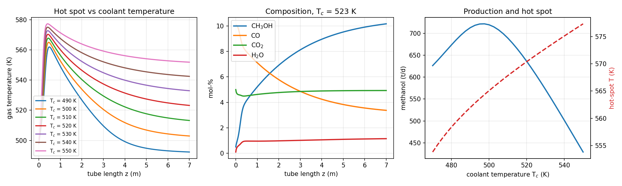
| Result, Tc = 523 K | Value |
|---|---|
| Hot spot | 571 K at 0.42 m |
| Outlet temperature | 526 K |
| CH₃OH at outlet | 10.2 % (equilibrium at 523 K: 10.7 %) |
| CO + CO₂ conversion per pass | 53.6 % |
| Methanol production | 803 kmol/h ≈ 620 t/d |
| Coolant temperature for maximum production | ≈ 498 K (≈ 720 t/d) |
With the same catalyst, the tube-cooled reactor makes about 70 % more methanol than the quench converter. Heat removal lets the gas follow the equilibrium curve downwards along the tube instead of stopping on it at a high temperature. The profiles show three features typical of all cooled, exothermic tubular reactors:
- A sharp hot spot near the inlet, where the gas is far from equilibrium and the rate is highest (Froment et al., 2011, Ch. 11). Its height is set mainly by the inlet composition and the tube diameter. The coolant temperature moves it by only a few kelvin here, but in less favourable cases it is the start of a runaway: near that limit the hot spot becomes extremely sensitive to small changes in coolant temperature or feed, which Bilous and Amundson called parametric sensitivity (Bilous & Amundson, 1956; Hlavacek et al., 2000, Sec. 4.4).
- Behind the hot spot, the gas cools towards the coolant temperature, and the outlet approaches the equilibrium composition at Tc. The coolant temperature therefore sets the final conversion.
- Production has an optimum coolant temperature. Colder is better for equilibrium until the catalyst becomes too slow. For fresh catalyst the optimum lies near 500 K. As the catalyst ages, operators raise the steam pressure to keep the rate up, which is why plants start their run at a low coolant temperature and end it at a high one (Fiedler et al., 2000, Sec. 4.2.4).
"""
Methanol synthesis — boiling-water-cooled multitubular reactor (Lurgi type)
bdrworks.org · Handbook · Methanol, worked model 2

Reactions on Cu/ZnO/Al2O3 (Vanden Bussche & Froment, 1996):
    1:  CO2 + 3 H2 <=> CH3OH + H2O
    2:  CO2 +   H2 <=> CO + H2O          (reverse water-gas shift)
One representative tube, 1-D pseudo-homogeneous plug flow, shell side at the
boiling temperature of the cooling water (constant Tc):
    dF_i/dz = rho_b A_t * sum_j nu_ij r_j
    (sum F_i cp_i) dT/dz = rho_b A_t * sum_j (-dH_j) r_j - U pi D (T - Tc)

Run:  python meoh_tubular.py      (needs numpy, scipy, matplotlib)
"""
import numpy as np
from scipy.integrate import solve_ivp
import matplotlib.pyplot as plt

# ---------------------------------------------------------------- data
SPECIES = ["CO", "CO2", "H2", "CH3OH", "H2O", "CH4", "N2"]
#                 CO   CO2   H2  MeOH  H2O  CH4  N2
NU = np.array([[0.0, -1.0, -3.0, 1.0, 1.0, 0.0, 0.0],     # 1: CO2 + 3H2 <=> CH3OH + H2O
               [1.0, -1.0, -1.0, 0.0, 1.0, 0.0, 0.0]])    # 2: CO2 + H2  <=> CO + H2O (RWGS)
RG = 8.314                                                 # J/(mol K)

# ideal-gas cp = A + B T + C T^2 + D T^3, J/(mol K)  (Reid, Prausnitz & Poling)
CP = np.array([[30.87, -1.285e-2, 2.789e-5, -1.272e-8],   # CO
               [19.80, 7.344e-2, -5.602e-5, 1.715e-8],    # CO2
               [27.14, 9.274e-3, -1.381e-5, 7.645e-9],    # H2
               [21.15, 7.092e-2, 2.587e-5, -2.852e-8],    # CH3OH
               [32.24, 1.924e-3, 1.055e-5, -3.596e-9],    # H2O
               [19.25, 5.213e-2, 1.197e-5, -1.132e-8],    # CH4
               [31.15, -1.357e-2, 2.680e-5, -1.168e-8]])  # N2
HF = np.array([-110.53, -393.51, 0.0, -200.94, -241.83, -74.87, 0.0]) * 1e3   # J/mol, 298.15 K


def cp(T):
    """Heat capacities of all species, J/(mol K)."""
    return CP @ np.array([1.0, T, T**2, T**3])


def h(T):
    """Molar enthalpies H_f(298) + integral of cp, J/mol."""
    T0 = 298.15
    dT = np.array([T - T0, (T**2 - T0**2) / 2, (T**3 - T0**3) / 3, (T**4 - T0**4) / 4])
    return HF + CP @ dT


def dH_rxn(T):
    """Heats of reaction 1 and 2, J/mol."""
    return NU @ h(T)


def K_eq(T):
    """Equilibrium constants (Graaf et al.), partial pressures in bar.
    K1 for CO2 + 3H2 = CH3OH + H2O (bar^-2);  K3 for CO + H2O = CO2 + H2 (-)."""
    K1 = 10.0 ** (3066.0 / T - 10.592)
    K3 = 10.0 ** (2073.0 / T - 2.029)
    return K1, K3


def rates(T, p):
    """Vanden Bussche & Froment (1996) rates, mol/(kg_cat s); p = partial pressures in bar."""
    pCO, pCO2, pH2, pM, pW = [max(x, 1e-10) for x in p[:5]]
    k = lambda A, B: A * np.exp(B / (RG * T))
    k1, k2, k3, k4, k5 = k(1.07, 36696), k(3453.38, 0), k(0.499, 17197), k(6.62e-11, 124119), k(1.22e10, -94765)
    K1, K3 = K_eq(T)
    den = 1.0 + k2 * pW / pH2 + k3 * np.sqrt(pH2) + k4 * pW
    r1 = k1 * pCO2 * pH2 * (1.0 - pW * pM / (K1 * pH2**3 * pCO2)) / den**3
    r2 = k5 * pCO2 * (1.0 - K3 * pW * pCO / (pCO2 * pH2)) / den
    return np.array([r1, r2])


def equilibrium(T, P, F):
    """Chemical equilibrium of reactions 1 and 2 from flows F (any unit); returns outlet flows."""
    from scipy.optimize import fsolve
    K1, K3 = K_eq(T)
    def res(x):
        n = F + NU.T @ x
        n = np.maximum(n, 1e-12)
        p = P * n / n.sum()
        return [np.log(p[3] * p[4] / (p[1] * p[2]**3)) - np.log(K1),
                np.log(p[0] * p[4] / (p[1] * p[2])) + np.log(K3)]
    x = fsolve(res, [0.1 * F.sum() * 0.05, 0.0], xtol=1e-12)
    return F + NU.T @ x

# ---------------------------------------------------------------- reactor
P = 75.0                  # bar
F0 = 10000.0              # total feed, kmol/h
Y0 = np.array([0.10, 0.05, 0.70, 0.005, 0.001, 0.12, 0.024])
Y0 = Y0 / Y0.sum()
T_IN = 498.0              # gas inlet, K
N_T = 5000                # number of tubes
D = 0.040                 # tube inside diameter, m
L = 7.0                   # tube length, m
RHO_B = 1140.0            # catalyst bulk density, kg/m3
U = 250.0                 # overall heat-transfer coefficient, W/(m2 K)
A_T = np.pi * D**2 / 4


def rhs(z, u, Tc):
    F, T = u[:7], u[7]                         # F in mol/s per tube
    p = P * F / F.sum()
    r = rates(T, p)                            # mol/(kg s)
    dF = RHO_B * A_T * (NU.T @ r)
    q = U * np.pi * D * (T - Tc)               # W per m of tube
    dT = (RHO_B * A_T * np.dot(-dH_rxn(T), r) - q) / np.dot(F, cp(T))
    return np.append(dF, dT)


def solve(Tc, T_in=T_IN, n=400):
    F_tube = F0 * 1000 / 3600 / N_T * Y0       # mol/s per tube
    sol = solve_ivp(rhs, (0, L), np.append(F_tube, T_in), args=(Tc,), method="LSODA",
                    rtol=1e-8, atol=1e-10, dense_output=True)
    z = np.linspace(0, L, n)
    return z, sol.sol(z)


def summary(u):
    F_in, F_out = u[:7, 0], u[:7, -1]
    meoh = (F_out[3] - F_in[3]) * N_T * 3600 / 1000          # kmol/h
    xc = 1 - (F_out[0] + F_out[1]) / (F_in[0] + F_in[1])      # carbon (CO+CO2) conversion
    return meoh, meoh * 32.04 * 24 / 1000, xc, F_out[3] / F_out.sum()


if __name__ == "__main__":
    Tc = 523.0                                               # boiling water at ~40 bar
    z, u = solve(Tc)
    meoh, tpd, xc, y = summary(u)
    print(f"P = {P:.0f} bar, feed {F0:.0f} kmol/h at {T_IN:.0f} K, coolant {Tc:.0f} K, "
          f"{N_T} tubes x {L} m, catalyst {RHO_B*A_T*L*N_T/1000:.1f} t")
    print(f"hot spot {u[7].max():.1f} K at z = {z[u[7].argmax()]:.2f} m, outlet {u[7,-1]:.1f} K")
    print(f"MeOH out {100*y:.2f} mol-%, CO+CO2 conversion {100*xc:.1f} %, "
          f"production {meoh:.0f} kmol/h = {tpd:.0f} t/d")

    # parametric sensitivity: coolant temperature
    Tcs = np.arange(490, 551, 10)
    fig, ax = plt.subplots(1, 3, figsize=(14, 4.2))
    for t in Tcs:
        zz, uu = solve(t)
        ax[0].plot(zz, uu[7], lw=1.8, label=f"T$_c$ = {t:.0f} K")
    ax[0].set(xlabel="tube length z (m)", ylabel="gas temperature (K)", title="Hot spot vs coolant temperature")
    ax[0].legend(fontsize=8)
    ax[1].plot(z, 100 * u[3] / u[:7].sum(axis=0), lw=2, label="CH$_3$OH")
    ax[1].plot(z, 100 * u[0] / u[:7].sum(axis=0), lw=2, label="CO")
    ax[1].plot(z, 100 * u[1] / u[:7].sum(axis=0), lw=2, label="CO$_2$")
    ax[1].plot(z, 100 * u[4] / u[:7].sum(axis=0), lw=2, label="H$_2$O")
    ax[1].set(xlabel="tube length z (m)", ylabel="mol-%", title=f"Composition, T$_c$ = {Tc:.0f} K")
    ax[1].legend()
    tc = np.arange(470, 551, 2.5)
    res = []
    for t in tc:
        uu = solve(t)[1]
        res.append(summary(uu) + (uu[7].max(),))
    best = tc[int(np.argmax([r[1] for r in res]))]
    print(f"coolant temperature for maximum production ≈ {best:.0f} K")
    ax[2].plot(tc, [r[1] for r in res], lw=2, c="C0")
    ax[2].set(xlabel="coolant temperature T$_c$ (K)", ylabel="methanol (t/d)", title="Production and hot spot")
    a2 = ax[2].twinx(); a2.plot(tc, [r[4] for r in res], lw=2, c="C3", ls="--"); a2.set_ylabel("hot-spot T (K)", color="C3")
    for a in ax:
        a.grid(alpha=0.3)
    fig.tight_layout()
    fig.savefig("meoh_tubular.png", dpi=150)
    plt.show()
function meoh_tubular()
% Methanol synthesis - boiling-water-cooled multitubular reactor (Lurgi type)
% bdrworks.org - Handbook - Methanol, worked model 2
%   dF/dz = rho_b A_t nu' r ,  (sum F cp) dT/dz = rho_b A_t sum(-dH r) - U pi D (T - Tc)
% Save as meoh_tubular.m and run:  meoh_tubular

p = params();
Tc = 523;
[z, u] = tube(p, Tc);
[meoh, tpd, xc, y] = summary(p, u);
[Tmax, i] = max(u(:,8));
fprintf('hot spot %.1f K at z = %.2f m, outlet %.1f K\n', Tmax, z(i), u(end,8));
fprintf('MeOH out %.2f mol-%%, CO+CO2 conversion %.1f %%, production %.0f kmol/h = %.0f t/d\n', 100*y, 100*xc, meoh, tpd);

% coolant temperature sweep
tc = 470:2.5:550;  prod = zeros(size(tc));  hs = prod;
for k = 1:numel(tc)
    [~, uk] = tube(p, tc(k));  [~, prod(k)] = summary(p, uk);  hs(k) = max(uk(:,8));
end
[~, ib] = max(prod);
fprintf('coolant temperature for maximum production = %.0f K\n', tc(ib));
figure('Position', [100 100 1000 380]);
subplot(1,2,1); plot(z, u(:,8), 'LineWidth', 2); xlabel('z (m)'); ylabel('T (K)'); grid on;
subplot(1,2,2); plot(tc, prod, 'LineWidth', 2); xlabel('T_c (K)'); ylabel('methanol (t/d)'); grid on;
end

function p = params()
p.P = 75;  p.F0 = 10000;  y0 = [0.10 0.05 0.70 0.005 0.001 0.12 0.024]';  p.y0 = y0/sum(y0);
p.Tin = 498;  p.Nt = 5000;  p.D = 0.040;  p.L = 7;  p.rho = 1140;  p.U = 250;  p.At = pi*p.D^2/4;
end

function [z, u] = tube(p, Tc)
f0 = p.F0*1000/3600/p.Nt*p.y0;                         % mol/s per tube
opts = odeset('RelTol', 1e-8, 'AbsTol', 1e-10);
[z, u] = ode45(@(z,u) rhs(u, p, Tc), linspace(0, p.L, 400), [f0; p.Tin], opts);
end

function du = rhs(u, p, Tc)
F = u(1:7);  T = u(8);  nu = stoich();
r = rates(T, p.P*F/sum(F));
du = [p.rho*p.At*(nu'*r);
      (p.rho*p.At*(-dH_rxn(T))'*r - p.U*pi*p.D*(T - Tc))/(F'*cp_all(T))];
end

function [meoh, tpd, xc, y] = summary(p, u)
Fi = u(1,1:7);  Fo = u(end,1:7);
meoh = (Fo(4) - Fi(4))*p.Nt*3.6;  tpd = meoh*32.04*24/1000;
xc = 1 - (Fo(1) + Fo(2))/(Fi(1) + Fi(2));  y = Fo(4)/sum(Fo);
end

% ================================================================ properties & kinetics
function nu = stoich()
%        CO  CO2  H2  MeOH H2O CH4 N2
nu = [    0  -1   -3   1    1   0   0;      % CO2 + 3H2 <=> CH3OH + H2O
          1  -1   -1   0    1   0   0];     % CO2 + H2  <=> CO + H2O
end

function c = cp_all(T)
% ideal-gas cp, J/(mol K) (Reid, Prausnitz & Poling)
C = cpdata();  c = C*[1; T; T^2; T^3];
end

function H = h_all(T)
% H_f(298) + integral of cp, J/mol
C = cpdata();  T0 = 298.15;
Hf = [-110.53; -393.51; 0; -200.94; -241.83; -74.87; 0]*1e3;
H = Hf + C*[T-T0; (T^2-T0^2)/2; (T^3-T0^3)/3; (T^4-T0^4)/4];
end

function C = cpdata()
C = [30.87 -1.285e-2  2.789e-5 -1.272e-8;    % CO
     19.80  7.344e-2 -5.602e-5  1.715e-8;    % CO2
     27.14  9.274e-3 -1.381e-5  7.645e-9;    % H2
     21.15  7.092e-2  2.587e-5 -2.852e-8;    % CH3OH
     32.24  1.924e-3  1.055e-5 -3.596e-9;    % H2O
     19.25  5.213e-2  1.197e-5 -1.132e-8;    % CH4
     31.15 -1.357e-2  2.680e-5 -1.168e-8];   % N2
end

function dH = dH_rxn(T)
dH = stoich()*h_all(T);                      % J/mol, reactions 1 and 2
end

function [K1, K3] = K_eq(T)
% Graaf et al.: K1 (bar^-2) for CO2 + 3H2 = CH3OH + H2O, K3 for CO + H2O = CO2 + H2
K1 = 10^(3066/T - 10.592);  K3 = 10^(2073/T - 2.029);
end

function r = rates(T, p)
% Vanden Bussche & Froment (1996), mol/(kg_cat s), p in bar [CO CO2 H2 MeOH H2O ...]
p = max(p, 1e-10);  RG = 8.314;
k = @(A, B) A*exp(B/(RG*T));
k1 = k(1.07, 36696); k2 = k(3453.38, 0); k3 = k(0.499, 17197); k4 = k(6.62e-11, 124119); k5 = k(1.22e10, -94765);
[K1, K3] = K_eq(T);
den = 1 + k2*p(5)/p(3) + k3*sqrt(p(3)) + k4*p(5);
r = [k1*p(2)*p(3)*(1 - p(5)*p(4)/(K1*p(3)^3*p(2)))/den^3;
     k5*p(2)*(1 - K3*p(5)*p(1)/(p(2)*p(3)))/den];
end
8Solution 3 · Synthesis loop
With 5–10 % methanol per pass, about half of the synthesis gas is converted before equilibrium is reached, so a plant cannot run once-through (Fiedler et al., 2000, Sec. 5.2). The reactor outlet is cooled to about 40 °C, methanol and water condense and are separated, and the unreacted gas is compressed back to the reactor. CH₄ and N₂ enter with the make-up gas and never react, and the excess hydrogen of a reformer gas has no partner. All of these would accumulate without limit, so a fraction φ of the separator gas is purged; the purge rate is set by the inert content and the stoichiometric number (Fiedler et al., 2000, Sec. 5.2).
The loop is a recycle problem. Guessing the recycle stream (the "tear stream") lets the reactor be calculated. The reactor outlet then gives a new recycle stream, and the guess must equal the result:
The Python code solves Eq. 7 as seven nonlinear equations with fsolve, a Newton-type method (Virtanen et al., 2020; Finlayson et al., 2006, Sec. 1.3). The MATLAB code uses the bounded Wegstein method, the classic acceleration used by flowsheet simulators, and needs no toolbox (Wegstein, 1958). Both give the same answer. In this model the separator is a perfect split: all methanol and water condense and no gas dissolves. A flash calculation with an equation of state would refine this.
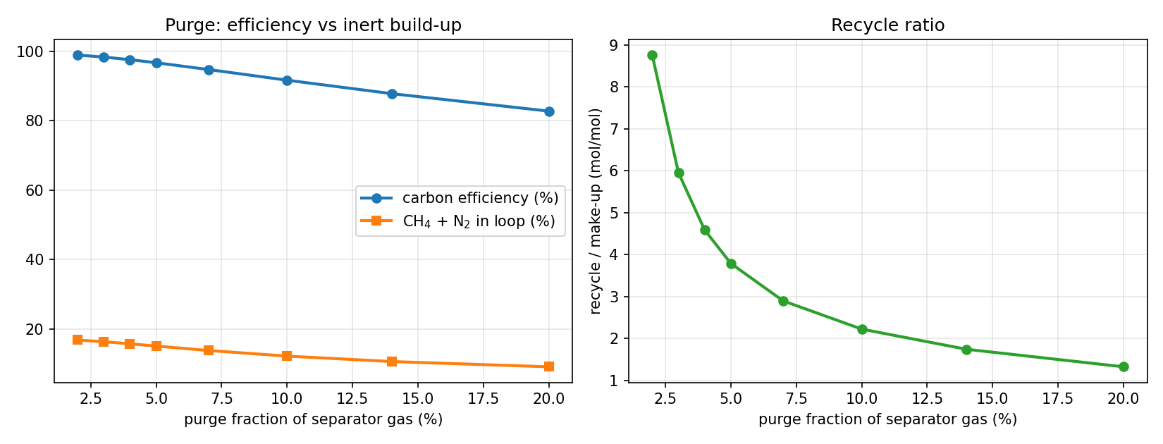
| Purge | Recycle / make-up | CH₄ + N₂ in loop | Methanol | Carbon efficiency |
|---|---|---|---|---|
| 2 % | 8.8 | 16.8 % | 476 t/d | 99.0 % |
| 5 % | 3.8 | 15.0 % | 465 t/d | 96.8 % |
| 10 % | 2.2 | 12.1 % | 441 t/d | 91.7 % |
| 20 % | 1.3 | 9.0 % | 398 t/d | 82.8 % |
The purge is an economic trade-off. A small purge recovers almost all carbon as methanol, but only by circulating a huge recycle stream: at 2 % purge, nine moles of gas circulate for every mole of make-up gas. Recycle compressor power, pipe and reactor sizes scale with this flow. A large purge keeps the loop small but burns valuable carbon oxides as fuel. Industrial loops settle at recycle ratios of about 3–5, which corresponds to the few-percent purge shown here. Note that the reactor in the loop sees a very different gas from the one in Solutions 1 and 2; its inlet is now an output of the calculation.
"""
Methanol synthesis loop — reactor, separator, recycle and purge
bdrworks.org · Handbook · Methanol, worked model 3

Make-up gas from the reformer is mixed with recycle gas and fed to the tube-cooled
reactor of model 2. The reactor outlet is cooled to 40 °C; methanol and water
condense (taken here as a perfect split), and the remaining gas is recycled.
A small purge keeps CH4 and N2 — which enter with the make-up gas and never
react — from accumulating without limit.

Unknowns: the recycle flows R_i (7 species).  Equations (tear stream):
    R = (1 - phi) * G( reactor( M + R ) )
where G keeps the gas species and phi is the purge fraction. Solved with fsolve.

Run:  python meoh_loop.py      (needs numpy, scipy, matplotlib)
"""
import numpy as np
from scipy.integrate import solve_ivp
from scipy.optimize import fsolve
import matplotlib.pyplot as plt

# ---------------------------------------------------------------- data
SPECIES = ["CO", "CO2", "H2", "CH3OH", "H2O", "CH4", "N2"]
#                 CO   CO2   H2  MeOH  H2O  CH4  N2
NU = np.array([[0.0, -1.0, -3.0, 1.0, 1.0, 0.0, 0.0],     # 1: CO2 + 3H2 <=> CH3OH + H2O
               [1.0, -1.0, -1.0, 0.0, 1.0, 0.0, 0.0]])    # 2: CO2 + H2  <=> CO + H2O (RWGS)
RG = 8.314                                                 # J/(mol K)

# ideal-gas cp = A + B T + C T^2 + D T^3, J/(mol K)  (Reid, Prausnitz & Poling)
CP = np.array([[30.87, -1.285e-2, 2.789e-5, -1.272e-8],   # CO
               [19.80, 7.344e-2, -5.602e-5, 1.715e-8],    # CO2
               [27.14, 9.274e-3, -1.381e-5, 7.645e-9],    # H2
               [21.15, 7.092e-2, 2.587e-5, -2.852e-8],    # CH3OH
               [32.24, 1.924e-3, 1.055e-5, -3.596e-9],    # H2O
               [19.25, 5.213e-2, 1.197e-5, -1.132e-8],    # CH4
               [31.15, -1.357e-2, 2.680e-5, -1.168e-8]])  # N2
HF = np.array([-110.53, -393.51, 0.0, -200.94, -241.83, -74.87, 0.0]) * 1e3   # J/mol, 298.15 K


def cp(T):
    """Heat capacities of all species, J/(mol K)."""
    return CP @ np.array([1.0, T, T**2, T**3])


def h(T):
    """Molar enthalpies H_f(298) + integral of cp, J/mol."""
    T0 = 298.15
    dT = np.array([T - T0, (T**2 - T0**2) / 2, (T**3 - T0**3) / 3, (T**4 - T0**4) / 4])
    return HF + CP @ dT


def dH_rxn(T):
    """Heats of reaction 1 and 2, J/mol."""
    return NU @ h(T)


def K_eq(T):
    """Equilibrium constants (Graaf et al.), partial pressures in bar.
    K1 for CO2 + 3H2 = CH3OH + H2O (bar^-2);  K3 for CO + H2O = CO2 + H2 (-)."""
    K1 = 10.0 ** (3066.0 / T - 10.592)
    K3 = 10.0 ** (2073.0 / T - 2.029)
    return K1, K3


def rates(T, p):
    """Vanden Bussche & Froment (1996) rates, mol/(kg_cat s); p = partial pressures in bar."""
    pCO, pCO2, pH2, pM, pW = [max(x, 1e-10) for x in p[:5]]
    k = lambda A, B: A * np.exp(B / (RG * T))
    k1, k2, k3, k4, k5 = k(1.07, 36696), k(3453.38, 0), k(0.499, 17197), k(6.62e-11, 124119), k(1.22e10, -94765)
    K1, K3 = K_eq(T)
    den = 1.0 + k2 * pW / pH2 + k3 * np.sqrt(pH2) + k4 * pW
    r1 = k1 * pCO2 * pH2 * (1.0 - pW * pM / (K1 * pH2**3 * pCO2)) / den**3
    r2 = k5 * pCO2 * (1.0 - K3 * pW * pCO / (pCO2 * pH2)) / den
    return np.array([r1, r2])


def equilibrium(T, P, F):
    """Chemical equilibrium of reactions 1 and 2 from flows F (any unit); returns outlet flows."""
    from scipy.optimize import fsolve
    K1, K3 = K_eq(T)
    def res(x):
        n = F + NU.T @ x
        n = np.maximum(n, 1e-12)
        p = P * n / n.sum()
        return [np.log(p[3] * p[4] / (p[1] * p[2]**3)) - np.log(K1),
                np.log(p[0] * p[4] / (p[1] * p[2])) + np.log(K3)]
    x = fsolve(res, [0.1 * F.sum() * 0.05, 0.0], xtol=1e-12)
    return F + NU.T @ x

# ---------------------------------------------------------------- reactor (as in model 2)
P = 75.0; T_IN = 498.0; TC = 523.0
N_T = 5000; D = 0.040; L = 7.0; RHO_B = 1140.0; U = 250.0
A_T = np.pi * D**2 / 4


def rhs(z, u):
    F, T = u[:7], u[7]
    r = rates(T, P * F / F.sum())
    dF = RHO_B * A_T * (NU.T @ r)
    dT = (RHO_B * A_T * np.dot(-dH_rxn(T), r) - U * np.pi * D * (T - TC)) / np.dot(F, cp(T))
    return np.append(dF, dT)


def reactor(F_in):
    """F_in in kmol/h (whole reactor) -> outlet flows kmol/h and hot-spot temperature."""
    f = F_in * 1000 / 3600 / N_T
    sol = solve_ivp(rhs, (0, L), np.append(f, T_IN), method="LSODA", rtol=1e-7, atol=1e-10)
    return sol.y[:7, -1] * N_T * 3600 / 1000, sol.y[7].max()


# ---------------------------------------------------------------- loop
M_FLOW = 2500.0                                    # make-up gas, kmol/h
M_Y = np.array([0.17, 0.08, 0.72, 0.0, 0.0, 0.02, 0.01])
M = M_FLOW * M_Y
GAS = np.array([1, 1, 1, 0, 0, 1, 1], dtype=float) # species that stay in the gas at 40 °C


def solve_loop(phi, R_guess):
    def tear(R):
        out, _ = reactor(M + R)
        return (1 - phi) * GAS * out - R
    R = fsolve(tear, R_guess, xtol=1e-9)
    out, Tmax = reactor(M + R)
    return R, out, Tmax


def report(phi, R, out):
    meoh = out[3]                                   # kmol/h condensed methanol
    c_in = M[0] + M[1]
    return dict(recycle_ratio=R.sum() / M_FLOW, meoh=meoh, tpd=meoh * 32.04 * 24 / 1000,
                carbon_eff=meoh / c_in, inerts=(R[5] + R[6]) / R.sum(), purge=phi * (GAS * out).sum())


if __name__ == "__main__":
    SN = (M_Y[2] - M_Y[1]) / (M_Y[0] + M_Y[1])
    print(f"make-up {M_FLOW:.0f} kmol/h, stoichiometric number SN = {SN:.2f}")
    R = 3.0 * M_FLOW * np.array([0.05, 0.04, 0.70, 0, 0, 0.15, 0.06])
    phi = 0.05
    R, out, Tmax = solve_loop(phi, R)
    d = report(phi, R, out)
    print(f"purge {100*phi:.0f} %: recycle ratio {d['recycle_ratio']:.2f}, inerts in loop {100*d['inerts']:.1f} %, "
          f"hot spot {Tmax:.1f} K")
    print(f"methanol {d['meoh']:.0f} kmol/h = {d['tpd']:.0f} t/d, carbon efficiency {100*d['carbon_eff']:.1f} %")

    # purge fraction sweep (continuation from the previous solution)
    phis = [0.02, 0.03, 0.04, 0.05, 0.07, 0.10, 0.14, 0.20]
    rows, Rg = [], R
    for ph in sorted(phis, key=lambda x: abs(x - phi)):
        Rg, o, Tm = solve_loop(ph, Rg)
        rows.append((ph, report(ph, Rg, o), Tm))
    rows.sort(key=lambda r: r[0])
    for ph, dd, Tm in rows:
        print(f"  purge {100*ph:4.0f} %: recycle {dd['recycle_ratio']:.2f}, inerts {100*dd['inerts']:5.1f} %, "
              f"{dd['tpd']:5.0f} t/d, carbon eff. {100*dd['carbon_eff']:.1f} %")

    fig, ax = plt.subplots(1, 2, figsize=(11, 4.2))
    x = [100 * r[0] for r in rows]
    ax[0].plot(x, [100 * r[1]["carbon_eff"] for r in rows], "o-", lw=2, label="carbon efficiency (%)")
    ax[0].plot(x, [100 * r[1]["inerts"] for r in rows], "s-", lw=2, label="CH$_4$ + N$_2$ in loop (%)")
    ax[0].set(xlabel="purge fraction of separator gas (%)", title="Purge: efficiency vs inert build-up"); ax[0].legend()
    ax[1].plot(x, [r[1]["recycle_ratio"] for r in rows], "o-", lw=2, c="C2")
    ax[1].set(xlabel="purge fraction of separator gas (%)", ylabel="recycle / make-up (mol/mol)", title="Recycle ratio")
    for a in ax:
        a.grid(alpha=0.3)
    fig.tight_layout()
    fig.savefig("meoh_loop.png", dpi=150)
    plt.show()
function meoh_loop()
% Methanol synthesis loop - reactor, separator, recycle and purge
% bdrworks.org - Handbook - Methanol, worked model 3
%   tear stream R = (1 - phi) * gas( reactor(M + R) ), solved by Wegstein iteration
% Save as meoh_loop.m and run:  meoh_loop

p.P = 75;  p.Tin = 498;  p.Tc = 523;  p.Nt = 5000;  p.D = 0.040;  p.L = 7;  p.rho = 1140;  p.U = 250;  p.At = pi*p.D^2/4;
My = [0.17 0.08 0.72 0 0 0.02 0.01]';  M = 2500*My;
gas = [1 1 1 0 0 1 1]';
phis = [0.02 0.03 0.04 0.05 0.07 0.10 0.14 0.20];
R = 3*2500*[0.05 0.04 0.70 0 0 0.15 0.06]';
fprintf('SN = %.2f\n', (My(3) - My(2))/(My(1) + My(2)));
for ph = phis
    g = @(R) (1 - ph)*gas.*reactor(M + R, p);
    R = wegstein(g, R);
    out = reactor(M + R, p);
    fprintf('purge %4.0f %%: recycle %.2f, inerts %.1f %%, %.0f t/d, carbon eff. %.1f %%\n', 100*ph, ...
        sum(R)/2500, 100*(R(6) + R(7))/sum(R), out(4)*32.04*24/1000, 100*out(4)/(M(1) + M(2)));
end
end

function x = wegstein(g, x)
% bounded Wegstein acceleration of the fixed-point iteration x = g(x)
gx = g(x);  x1 = gx;
for it = 1:200
    gx1 = g(x1);
    s = (gx1 - gx)./(x1 - x + 1e-12);  q = s./(s - 1);  q = min(max(q, -5), 0);
    x = x1;  gx = gx1;  x1 = q.*x + (1 - q).*gx;
    if norm(x1 - x) < 1e-6*norm(x), break; end
end
x = x1;
end

function out = reactor(Fin, p)
f = Fin*1000/3600/p.Nt;
opts = odeset('RelTol', 1e-7, 'AbsTol', 1e-10);
[~, u] = ode45(@(z,u) rhs(u, p), [0 p.L], [f; p.Tin], opts);
out = u(end,1:7)'*p.Nt*3.6;
end

function du = rhs(u, p)
F = u(1:7);  T = u(8);  nu = stoich();
r = rates(T, p.P*F/sum(F));
du = [p.rho*p.At*(nu'*r);
      (p.rho*p.At*(-dH_rxn(T))'*r - p.U*pi*p.D*(T - p.Tc))/(F'*cp_all(T))];
end

% ================================================================ properties & kinetics
function nu = stoich()
%        CO  CO2  H2  MeOH H2O CH4 N2
nu = [    0  -1   -3   1    1   0   0;      % CO2 + 3H2 <=> CH3OH + H2O
          1  -1   -1   0    1   0   0];     % CO2 + H2  <=> CO + H2O
end

function c = cp_all(T)
% ideal-gas cp, J/(mol K) (Reid, Prausnitz & Poling)
C = cpdata();  c = C*[1; T; T^2; T^3];
end

function H = h_all(T)
% H_f(298) + integral of cp, J/mol
C = cpdata();  T0 = 298.15;
Hf = [-110.53; -393.51; 0; -200.94; -241.83; -74.87; 0]*1e3;
H = Hf + C*[T-T0; (T^2-T0^2)/2; (T^3-T0^3)/3; (T^4-T0^4)/4];
end

function C = cpdata()
C = [30.87 -1.285e-2  2.789e-5 -1.272e-8;    % CO
     19.80  7.344e-2 -5.602e-5  1.715e-8;    % CO2
     27.14  9.274e-3 -1.381e-5  7.645e-9;    % H2
     21.15  7.092e-2  2.587e-5 -2.852e-8;    % CH3OH
     32.24  1.924e-3  1.055e-5 -3.596e-9;    % H2O
     19.25  5.213e-2  1.197e-5 -1.132e-8;    % CH4
     31.15 -1.357e-2  2.680e-5 -1.168e-8];   % N2
end

function dH = dH_rxn(T)
dH = stoich()*h_all(T);                      % J/mol, reactions 1 and 2
end

function [K1, K3] = K_eq(T)
% Graaf et al.: K1 (bar^-2) for CO2 + 3H2 = CH3OH + H2O, K3 for CO + H2O = CO2 + H2
K1 = 10^(3066/T - 10.592);  K3 = 10^(2073/T - 2.029);
end

function r = rates(T, p)
% Vanden Bussche & Froment (1996), mol/(kg_cat s), p in bar [CO CO2 H2 MeOH H2O ...]
p = max(p, 1e-10);  RG = 8.314;
k = @(A, B) A*exp(B/(RG*T));
k1 = k(1.07, 36696); k2 = k(3453.38, 0); k3 = k(0.499, 17197); k4 = k(6.62e-11, 124119); k5 = k(1.22e10, -94765);
[K1, K3] = K_eq(T);
den = 1 + k2*p(5)/p(3) + k3*sqrt(p(3)) + k4*p(5);
r = [k1*p(2)*p(3)*(1 - p(5)*p(4)/(K1*p(3)^3*p(2)))/den^3;
     k5*p(2)*(1 - K3*p(5)*p(1)/(p(2)*p(3)))/den];
end
9Comparison
| Configuration (50 t catalyst, 75 bar) | CH₃OH out | Production | Hottest point | Heat goes to |
|---|---|---|---|---|
| 1 · Four quench beds | 5.8 % | ≈ 370 t/d | 581 K | Cold feed (diluted product) |
| 2 · Boiling-water tubes, 523 K | 10.2 % | ≈ 620 t/d | 571 K | Medium-pressure steam |
| 3 · Loop with tube reactor, 5 % purge | — | ≈ 465 t/d from 2 500 kmol/h make-up | 556 K | Steam; carbon efficiency 97 % |
Solutions 1 and 2 answer a reactor question with a fixed feed. Solution 3 answers the plant question: with a given amount of synthesis gas, how much methanol comes out? That depends on the reactor, but just as much on the recycle and purge. The same pattern holds for ammonia, and for nearly every equilibrium-limited process.
10Try it
The tube-cooled reactor and the quench converter, ported to JavaScript with the same kinetics, run below. Try raising the coolant temperature until the hot spot passes 573 K, or feed a gas with less CO₂ and see the rate collapse.
11Going further
- Add the Ergun pressure drop to the tube model. Lurgi tubes lose a few bar, which lowers equilibrium conversion at the outlet.
- Replace the perfect separator in Solution 3 with a Peng–Robinson flash at 313 K and 72 bar, and follow the methanol that stays in the recycle gas and the gases dissolved in the crude methanol.
- Optimise the coolant temperature and the purge fraction together for maximum profit, counting purge gas as fuel and compressor power as cost.
- Model the two-stage Lurgi MegaMethanol arrangement: a water-cooled reactor followed by a gas-cooled reactor in which the cold feed flows through the tubes, as in a counter-current cooled converter.
- Add a catalyst deactivation law, a(t), and simulate a three-year run at constant production by adjusting Tc.
12References
- Bilous, O., & Amundson, N. R. (1956). Chemical reactor stability and sensitivity. II. Effect of parameters on sensitivity of empty tubular reactors. AIChE J., 2, 117–126.
- Brent, R. P. (1973). Algorithms for Minimization without Derivatives. Prentice-Hall, Englewood Cliffs, NJ.
- Chinchen, G. C., Denny, P. J., Parker, D. G., Spencer, M. S., & Whan, D. A. (1987). Mechanism of methanol synthesis from CO2/CO/H2 mixtures over copper/zinc oxide/alumina catalysts: use of 14C-labelled reactants. Appl. Catal., 30, 333–338.
- Fiedler, E., Grossmann, G., Kersebohm, D. B., Weiss, G., & Witte, C. (2000). Methanol. In Ullmann's Encyclopedia of Industrial Chemistry. Wiley-VCH, Weinheim. doi:10.1002/14356007.a16_465
- Finlayson, B. A., Biegler, L. T., & Grossmann, I. E. (2006). Mathematics in chemical engineering. In Ullmann's Encyclopedia of Industrial Chemistry. Wiley-VCH, Weinheim. doi:10.1002/14356007.b01_01.pub2
- Froment, G. F., Bischoff, K. B., & De Wilde, J. (2011). Chemical Reactor Analysis and Design (3rd ed.). Wiley, Hoboken, NJ.
- Graaf, G. H., Sijtsema, P. J. J. M., Stamhuis, E. J., & Joosten, G. E. H. (1986). Chemical equilibria in methanol synthesis. Chem. Eng. Sci., 41, 2883–2890.
- Hlavacek, V., Puszynski, J. A., Viljoen, H. J., & Gatica, J. E. (2000). Model reactors and their design equations. In Ullmann's Encyclopedia of Industrial Chemistry. Wiley-VCH, Weinheim. doi:10.1002/14356007.b04_121
- Linstrom, P. J. (Ed.), & Mallard, W. G. (Ed.) (2023). NIST Chemistry WebBook, NIST Standard Reference Database 69 (thermophysical and Shomate data). National Institute of Standards and Technology, Gaithersburg, MD.
- Poling, B. E., Prausnitz, J. M., & O'Connell, J. P. (2001). The Properties of Gases and Liquids (5th ed.). McGraw-Hill, New York.
- Smith, J. M., Van Ness, H. C., Abbott, M. M., & Swihart, M. T. (2018). Introduction to Chemical Engineering Thermodynamics (8th ed.). McGraw-Hill Education, New York.
- Vanden Bussche, K. M., & Froment, G. F. (1996). A steady-state kinetic model for methanol synthesis and the water gas shift reaction on a commercial Cu/ZnO/Al2O3 catalyst. J. Catal., 161, 1–10.
- Virtanen, P., Gommers, R., Oliphant, T. E., et al. (2020). SciPy 1.0: fundamental algorithms for scientific computing in Python. Nat. Methods, 17, 261–272.
- Wegstein, J. H. (1958). Accelerating convergence of iterative processes. Commun. ACM, 1(6), 9–13.
The converter sizes, gas compositions and heat-transfer coefficient are round numbers chosen for teaching, not data from a specific plant. The kinetic and equilibrium constants are from the open literature cited above.