1The problem
Almost all nitric acid is made by the Ostwald process: ammonia is burnt with air to nitrogen monoxide on a precious-metal gauze, the NO is oxidised to NO₂ in the gas phase, and the NO₂ is absorbed in water (Thiemann et al., 2000, Sec. 1.3). The three steps have very different engineering characters. The first is one of the fastest catalytic reactions in industry and is controlled by mass transfer to the gauze; the second is a slow homogeneous third-order reaction whose rate falls as the temperature rises; the third is a gas–liquid reaction with mass transfer on the trays of a column (Thiemann et al., 2000, Secs. 1.3.1 and 1.3.2).
This page works through the first two steps and the gas train that joins them, with the plant numbers of the dual-pressure flow sheet in Ullmann's Encyclopedia as the case (Thiemann et al., 2000, Sec. 1.3.4.1 and Fig. 29). Each solution is written in Python and in MATLAB; the two versions give the same numbers, and the MATLAB files also run in GNU Octave.
2The Ostwald process
Plants are classified by the pressures of combustion and absorption. Monopressure plants burn and absorb at the same pressure, either medium (230–600 kPa) or high (700–1100 kPa); dual-pressure plants burn at 400–600 kPa and absorb at 900–1400 kPa, which combines the better combustion yield at moderate pressure with the smaller, more efficient absorption at high pressure (Thiemann et al., 2000, Sec. 1.3). In Europe the dual-pressure design is preferred for large plants, which today reach about 2000 t/d of acid in a single train (Thiemann et al., 2000, Sec. 1.3.4.1).
In the plant used here, ammonia evaporated at about 0.65 MPa is heated to 150 °C and mixed with about 86 % of the compressed air (the primary air). The mixture, at about 220 °C and 10 % NH₃, burns on the gauze at 890 °C with a 96.5 % yield of NO. The waste-heat boiler cools the gas to 355 °C while raising high-pressure steam. The gas then passes through piping for oxidation, a tail-gas preheater, more piping, an economizer, a second tail-gas preheater, a feed-water preheater and two cooler–condensers, where the water of combustion condenses as 43–52 % acid. The remaining air (the secondary air) strips dissolved NOₓ from the product acid in the bleacher and joins the nitrous gas before the nitrous-gas compressor raises it to 1.1 MPa; after a last cooler–condenser at 50 °C the gas, now at least 90 % oxidised, enters the absorption tower (Thiemann et al., 2000, Sec. 1.3.4.1). The tail gas is reheated to 350 °C by the nitrous gas and expanded in a turbine that supplies about two thirds of the compressor power (Thiemann et al., 2000, Sec. 1.3.4.1). This is why the heat of NO oxidation is recovered at as high a temperature as possible, a point Solution 3 returns to.
3Chemistry and data
On the gauze, 93–98 % of the ammonia is converted to NO; the rest forms mainly nitrogen and some N₂O (Thiemann et al., 2000, Sec. 1.3.1, Eqs. 4–6). The models keep the main reaction and lump the losses into the nitrogen reaction:
Downstream of the gauze the chemistry is homogeneous. NO is oxidised by the remaining oxygen, and the NO₂ dimerises to N₂O₄ and combines with NO to N₂O₃; both association reactions are so fast that they can be treated as equilibria. The absorption step converts NO₂ (in practice mostly N₂O₄) to nitric acid and releases one NO for every three NO₂, which has to be oxidised again in the tower (Thiemann et al., 2000, Sec. 1.3.2, Eqs. 2, 3 and 10–12):
The oxidation of NO is one of the few known homogeneous third-order gas reactions (Thiemann et al., 2000, Sec. 1.3; Davis & Davis, 2003, Table 1.4.3). Its rate follows the third-order equation going back to Bodenstein, written with partial pressures in atm and with the rate constant in the form given by Thiemann et al. (Bodenstein, 1922; Thiemann et al., 2000, Sec. 1.3.2, Eqs. 13 and 14):
Here r is the rate of oxygen consumption per unit gas volume, so NO disappears twice as fast (Fogler, 2016, Ch. 3). The constant falls as the temperature rises: from 14.1 atm⁻²s⁻¹ at 25 °C to 1.0 at 350 °C. This negative temperature coefficient is the defining feature of the reaction (Thiemann et al., 2000, Sec. 1.3.2). As a check, the termolecular rate constant tabulated by Davis and Davis, 3.3 × 10⁻³⁹ exp(530/T) cm⁶ molecule⁻² s⁻¹, converts to 11.8 atm⁻²s⁻¹ at 25 °C and to within 10 % of Eq. 5 between 100 and 350 °C (Davis & Davis, 2003, Table 1.4.3).
Ullmann's Eq. 13 has no reverse term, which is correct below about 200 °C. The models add one so that the rate falls to zero at equilibrium, with Kox computed from the standard Gibbs energies of NO, O₂ and NO₂ (Smith et al., 2018, Secs. 14.3 and 14.4). It gives Kox = 2.3 × 10¹² atm⁻¹ at 25 °C but only 158 atm⁻¹ at 600 K, so the reverse reaction matters in the hot end of the gas train. The dimer equilibria are taken from the same source (Thiemann et al., 2000, Sec. 1.3.2, Eqs. 17 and 19; Hoftyzer & Kwanten, 1972):
Enthalpies, heat capacities and Gibbs energies of NH₃, O₂, N₂, NO, NO₂ and H₂O come from the NASA seven-coefficient polynomials of the GRI-Mech 3.0 data set (Smith et al., 1999; Gordon & McBride, 1994). They reproduce the heats of reaction in Ullmann's equations: −902 kJ for Eq. 1 at 25 °C against −904 kJ, and −114 kJ per mol O₂ for NO oxidation (Thiemann et al., 2000, Sec. 1.3.2, Eq. 10).
4Solution 1 · The ammonia burner
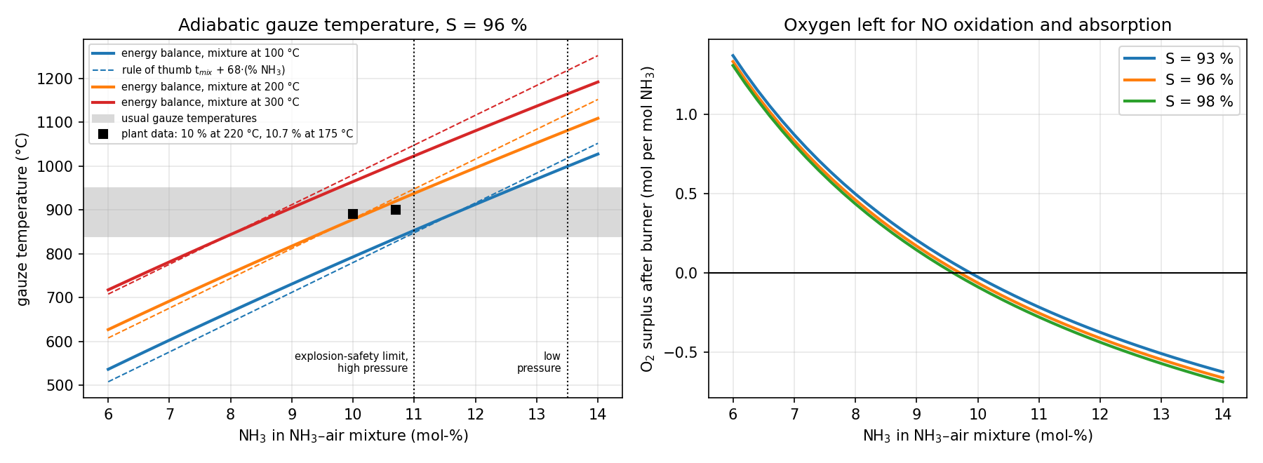
The gauze is thin and the reaction is complete within a few millimetres, so the burner can be treated as an adiabatic reactor with complete conversion of ammonia. With the NO selectivity S as a parameter, the outlet flows follow from Eq. 1, and the gauze temperature from the energy balance between the inlet mixture and the product gas (Smith et al., 2018, Sec. 4.7):
The code solves Eq. 3 for Tg with Brent's method (Brent, 1973). Ullmann gives a rule of thumb for the same balance, a rise of about 68 K for every per cent of ammonia in the mixture (Thiemann et al., 2000, Sec. 1.3.1, Eq. 9):
| Case | Model | Rule, Eq. 4 | Plant |
|---|---|---|---|
| 10 % NH₃, mixture at 100 °C, S = 96 % | 793 °C | 780 °C | — |
| 10 % NH₃, mixture at 200 °C, S = 96 % | 878 °C | 880 °C | — |
| 10 % NH₃, mixture at 300 °C, S = 96 % | 965 °C | 980 °C | — |
| Dual-pressure plant: 10 % at 220 °C, S = 96.5 % | 894 °C | 900 °C | 890 °C |
| High-pressure plant: 10.7 % at 175 °C | 899 °C | 903 °C | ca. 900 °C |
The energy balance and the rule agree within 15 K, and both reproduce the plant temperatures of the flow sheets (Thiemann et al., 2000, Sec. 1.3.4.1). Averaged from 0 to 10 % NH₃ with the mixture at 200 °C, the model gives 67.8 K per per cent, the rule's 68 K. The local slope is not constant, though: it falls from about 64 to 56 K per per cent between 7 and 13 % NH₃, because the heat capacity of the product gas rises with temperature, so the rule overestimates hot, rich mixtures. The usual gauze temperatures are 840–850 °C at 0.1–0.2 MPa, 880–900 °C at 0.3–0.7 MPa and 900–950 °C at 0.8–1.2 MPa (Thiemann et al., 2000, Table 3). Higher temperatures improve the conversion but raise the platinum loss steeply, so the operator sets the temperature, and through Eq. 4 the ammonia ratio, as a compromise (Thiemann et al., 2000, Sec. 1.3.1, Figs. 4 and 5).
The ammonia content is limited from above by safety. Stoichiometry would allow 14.38 % NH₃ in air, but ammonia–air mixtures are explosive, mixing is never perfect and the explosion limit falls with pressure: high-pressure burners work with up to about 11 % and low-pressure burners up to 13.5 % (Thiemann et al., 2000, Sec. 1.3.1 and Table 2). The right panel of Figure 1 shows a second, less obvious limit. The overall reaction NH₃ + 2 O₂ → HNO₃ + H₂O needs two moles of oxygen per mole of ammonia, so above about 9.7 % NH₃ (for S = 96 %) the primary air cannot supply all the oxygen the absorption needs. At 10 % the deficit is 0.065 mol O₂ per mol NH₃. This is the reason for the secondary air: the dual-pressure flow sheet sends about 14 % of the air through the bleacher and adds it to the nitrous gas before absorption (Thiemann et al., 2000, Sec. 1.3.4.1). With that air, complete absorption of the NO would still leave about 2.8 % O₂ in the tail gas.
| Gas leaving the gauze (10 % NH₃, S = 96 %) | mol-% |
|---|---|
| NO | 9.37 |
| O₂ | 6.40 |
| H₂O | 14.63 |
| N₂ (with Ar) | 69.60 |
"""
Nitric acid — ammonia burner (catalytic oxidation of NH3 on Pt–Rh gauze)
bdrworks.org · Handbook · Nitric acid, worked model 1

Adiabatic energy balance of the gauze reactor:
    4 NH3 + 5 O2 -> 4 NO + 6 H2O   (selectivity S)
    4 NH3 + 3 O2 -> 2 N2 + 6 H2O   (the rest)
The gauze temperature follows from H_in(T_mix) = H_out(T_gauze); the oxygen balance
shows how much secondary air the absorption section needs.

Run:  python hno3_burner.py      (needs numpy, scipy, matplotlib)
"""
import numpy as np
from scipy.optimize import brentq
import matplotlib.pyplot as plt

# ---------------------------------------------------------------- data
SPECIES = ["NH3", "O2", "N2", "NO", "H2O"]
RG = 8.314                                   # J/(mol K)
Y_O2_AIR = 0.2095                            # O2 in dry air (Ar lumped with N2)

# NASA 7-coefficient polynomials (GRI-Mech 3.0 thermodynamic data): [T < 1000 K], [T > 1000 K]
NASA_LO = np.array([
    [4.28602740e+00, -4.66052300e-03, 2.17185130e-05, -2.28088870e-08, 8.26380460e-12, -6.74172850e+03, -6.25372770e-01],   # NH3
    [3.78245636e+00, -2.99673416e-03, 9.84730201e-06, -9.68129509e-09, 3.24372837e-12, -1.06394356e+03, 3.65767573e+00],   # O2
    [3.29867700e+00, 1.40824040e-03, -3.96322200e-06, 5.64151500e-09, -2.44485400e-12, -1.02089990e+03, 3.95037200e+00],   # N2
    [4.21847630e+00, -4.63897600e-03, 1.10410220e-05, -9.33613540e-09, 2.80357700e-12, 9.84462300e+03, 2.28084640e+00],    # NO
    [4.19864056e+00, -2.03643410e-03, 6.52040211e-06, -5.48797062e-09, 1.77197817e-12, -3.02937267e+04, -8.49032208e-01],  # H2O
])
NASA_HI = np.array([
    [2.63445210e+00, 5.66625600e-03, -1.72786760e-06, 2.38671610e-10, -1.25787860e-14, -6.54469580e+03, 6.56629280e+00],   # NH3
    [3.28253784e+00, 1.48308754e-03, -7.57966669e-07, 2.09470555e-10, -2.16717794e-14, -1.08845772e+03, 5.45323129e+00],   # O2
    [2.92664000e+00, 1.48797680e-03, -5.68476000e-07, 1.00970380e-10, -6.75335100e-15, -9.22797700e+02, 5.98052800e+00],   # N2
    [3.26060560e+00, 1.19110430e-03, -4.29170480e-07, 6.94576690e-11, -4.03360990e-15, 9.92097460e+03, 6.36930270e+00],    # NO
    [3.03399249e+00, 2.17691804e-03, -1.64072518e-07, -9.70419870e-11, 1.68200992e-14, -3.00042971e+04, 4.96677010e+00],   # H2O
])


def h(T):
    """Molar enthalpies including heats of formation, J/mol."""
    a = NASA_LO if T < 1000.0 else NASA_HI
    return RG * T * (a[:, 0] + a[:, 1]*T/2 + a[:, 2]*T**2/3 + a[:, 3]*T**3/4 + a[:, 4]*T**4/5 + a[:, 5]/T)


def feed(y_nh3, hum=0.0):
    """1 mol of NH3-air mixture; hum = mol H2O per mol dry air."""
    air = 1.0 - y_nh3
    dry = air / (1.0 + hum)
    return np.array([y_nh3, Y_O2_AIR * dry, (1 - Y_O2_AIR) * dry, 0.0, air - dry])


def burn(n0, S):
    """Outlet moles for complete NH3 conversion with NO selectivity S."""
    a = n0[0]
    return n0 + np.array([-a, -a * (1.25 * S + 0.75 * (1 - S)), 0.5 * a * (1 - S), a * S, 1.5 * a])


def gauze_temperature(y_nh3, T_mix, S=0.96, hum=0.0):
    n0 = feed(y_nh3, hum)
    n1 = burn(n0, S)
    H_in = n0 @ h(T_mix)
    return brentq(lambda T: n1 @ h(T) - H_in, T_mix, 2500.0), n1


if __name__ == "__main__":
    ys = np.linspace(0.06, 0.14, 41)
    fig, ax = plt.subplots(1, 2, figsize=(12, 4.4))
    for tmix, c in [(100, "tab:blue"), (200, "tab:orange"), (300, "tab:red")]:
        T = [gauze_temperature(y, tmix + 273.15)[0] - 273.15 for y in ys]
        ax[0].plot(100 * ys, T, lw=2, color=c, label=f"energy balance, mixture at {tmix} °C")
        ax[0].plot(100 * ys, tmix + 68 * 100 * ys, "--", color=c, lw=1, label="rule of thumb t$_{mix}$ + 68·(% NH$_3$)" if tmix == 100 else None)
    ax[0].axhspan(840, 950, color="0.85", zorder=0, label="usual gauze temperatures")
    ax[0].plot([10.0, 10.7], [890, 900], "ks", ms=6, label="plant data: 10 % at 220 °C, 10.7 % at 175 °C")
    ax[0].axvline(11.0, color="k", ls=":", lw=1); ax[0].axvline(13.5, color="k", ls=":", lw=1)
    ax[0].text(10.9, 530, "explosion-safety limit,\nhigh pressure", fontsize=7, ha="right"); ax[0].text(13.4, 530, "low\npressure", fontsize=7, ha="right")
    ax[0].set(xlabel="NH$_3$ in NH$_3$–air mixture (mol-%)", ylabel="gauze temperature (°C)", title="Adiabatic gauze temperature, S = 96 %")
    ax[0].legend(fontsize=7, loc="upper left"); ax[0].grid(alpha=0.3)
    # oxygen balance: O2 left after the burner vs O2 still needed for 4 NO + 3 O2 + 2 H2O -> 4 HNO3
    for S in [0.93, 0.96, 0.98]:
        left, need = [], []
        for y in ys:
            n1 = burn(feed(y), S)
            left.append(n1[1] / y); need.append(0.75 * n1[3] / y)
        ax[1].plot(100 * ys, np.array(left) - np.array(need), lw=2, label=f"S = {100*S:.0f} %")
    ax[1].axhline(0, color="k", lw=1)
    ax[1].set(xlabel="NH$_3$ in NH$_3$–air mixture (mol-%)", ylabel="O$_2$ surplus after burner (mol per mol NH$_3$)",
              title="Oxygen left for NO oxidation and absorption")
    ax[1].legend(); ax[1].grid(alpha=0.3)
    fig.tight_layout(); fig.savefig("hno3_burner.png", dpi=150)
    for tmix in [100, 200, 300]:
        T, n1 = gauze_temperature(0.10, tmix + 273.15)
        y = n1 / n1.sum()
        print(f"10 % NH3, mixture {tmix} °C: gauze {T-273.15:.0f} °C (rule {tmix+680:.0f} °C); outlet NO {100*y[3]:.2f} %, O2 {100*y[1]:.2f} %, H2O {100*y[4]:.2f} %")
    for y, tmix, S, T_plant in [(0.10, 220, 0.965, 890), (0.107, 175, 0.96, 900)]:
        T, n1 = gauze_temperature(y, tmix + 273.15, S)
        print(f"plant check: {100*y:.1f} % NH3 at {tmix} °C, S = {S}: model {T-273.15:.0f} °C, plant ca. {T_plant} °C")
    for S in [0.93, 0.96, 0.98]:
        n1 = burn(feed(0.10), S)
        print(f"S = {S:.2f}: O2 surplus after burner = {(n1[1] - 0.75*n1[3])/0.10:+.3f} mol O2 per mol NH3")
    plt.show()
function hno3_burner()
% Nitric acid - ammonia burner (Pt-Rh gauze), adiabatic energy balance
% bdrworks.org - Handbook - Nitric acid, worked model 1
%   4 NH3 + 5 O2 -> 4 NO + 6 H2O  (selectivity S),  4 NH3 + 3 O2 -> 2 N2 + 6 H2O  (rest)
%   H_in(T_mix) = H_out(T_gauze)
% Save as hno3_burner.m and run:  hno3_burner      (MATLAB or GNU Octave)

ys = linspace(0.06, 0.14, 41);
figure('Position',[100 100 1100 400]);
subplot(1,2,1); hold on;
cols = {'b','m','r'};  tm = [100 200 300];
for k = 1:3
    T = arrayfun(@(y) gauze_temperature(y, tm(k) + 273.15, 0.96), ys) - 273.15;
    plot(100*ys, T, cols{k}, 'LineWidth', 2);
    plot(100*ys, tm(k) + 68*100*ys, [cols{k} '--']);
end
plot([10 10.7], [890 900], 'ks', 'MarkerFaceColor', 'k');
plot([11 11], [500 1250], 'k:'); plot([13.5 13.5], [500 1250], 'k:');
xlabel('NH_3 in NH_3-air mixture (mol-%)'); ylabel('gauze temperature (\circC)');
title('Adiabatic gauze temperature, S = 96 %'); grid on;
legend('mix 100 \circC','rule t_{mix}+68(%NH_3)','mix 200 \circC','','mix 300 \circC','','plant data','Location','northwest');

subplot(1,2,2); hold on;
for S = [0.93 0.96 0.98]
    sur = arrayfun(@(y) o2_surplus(y, S), ys);
    plot(100*ys, sur, 'LineWidth', 2);
end
plot([6 14], [0 0], 'k');
xlabel('NH_3 in NH_3-air mixture (mol-%)'); ylabel('O_2 surplus after burner (mol per mol NH_3)');
title('Oxygen left for NO oxidation and absorption'); legend('S = 93 %','S = 96 %','S = 98 %'); grid on;

for t = tm
    [T, n1] = gauze_temperature(0.10, t + 273.15, 0.96);  y = n1/sum(n1);
    fprintf('10 %% NH3, mixture %d C: gauze %.0f C (rule %.0f C); NO %.2f %%, O2 %.2f %%, H2O %.2f %%\n', ...
            t, T - 273.15, t + 680, 100*y(4), 100*y(2), 100*y(5));
end
[T1] = gauze_temperature(0.10, 220 + 273.15, 0.965);
[T2] = gauze_temperature(0.107, 175 + 273.15, 0.96);
fprintf('plant check: 10 %% at 220 C -> %.0f C (plant ca. 890); 10.7 %% at 175 C -> %.0f C (plant ca. 900)\n', T1 - 273.15, T2 - 273.15);
for S = [0.93 0.96 0.98]
    fprintf('S = %.2f: O2 surplus after burner = %+.3f mol O2 per mol NH3\n', S, o2_surplus(0.10, S));
end
end

% ---------------------------------------------------------------- model
function n = feed(y)
% 1 mol NH3-air mixture: NH3, O2, N2, NO, H2O
air = 1 - y;
n = [y; 0.2095*air; 0.7905*air; 0; 0];
end

function n1 = burn(n0, S)
a = n0(1);
n1 = n0 + [-a; -a*(1.25*S + 0.75*(1 - S)); 0.5*a*(1 - S); a*S; 1.5*a];
end

function [T, n1] = gauze_temperature(y, Tmix, S)
n0 = feed(y);  n1 = burn(n0, S);
Hin = n0'*h_all(Tmix);
T = fzero(@(T) n1'*h_all(T) - Hin, [Tmix 2500]);
end

function s = o2_surplus(y, S)
n1 = burn(feed(y), S);
s = (n1(2) - 0.75*n1(4))/y;      % O2 left minus O2 needed for 4 NO + 3 O2 + 2 H2O -> 4 HNO3
end

% ---------------------------------------------------------------- NASA 7-coefficient polynomials (GRI-Mech 3.0)
function hh = h_all(T)
% molar enthalpies incl. heats of formation, J/mol: NH3, O2, N2, NO, H2O
lo = [4.28602740e+00 -4.66052300e-03 2.17185130e-05 -2.28088870e-08 8.26380460e-12 -6.74172850e+03 -6.25372770e-01
      3.78245636e+00 -2.99673416e-03 9.84730201e-06 -9.68129509e-09 3.24372837e-12 -1.06394356e+03 3.65767573e+00
      3.29867700e+00 1.40824040e-03 -3.96322200e-06 5.64151500e-09 -2.44485400e-12 -1.02089990e+03 3.95037200e+00
      4.21847630e+00 -4.63897600e-03 1.10410220e-05 -9.33613540e-09 2.80357700e-12 9.84462300e+03 2.28084640e+00
      4.19864056e+00 -2.03643410e-03 6.52040211e-06 -5.48797062e-09 1.77197817e-12 -3.02937267e+04 -8.49032208e-01];
hi = [2.63445210e+00 5.66625600e-03 -1.72786760e-06 2.38671610e-10 -1.25787860e-14 -6.54469580e+03 6.56629280e+00
      3.28253784e+00 1.48308754e-03 -7.57966669e-07 2.09470555e-10 -2.16717794e-14 -1.08845772e+03 5.45323129e+00
      2.92664000e+00 1.48797680e-03 -5.68476000e-07 1.00970380e-10 -6.75335100e-15 -9.22797700e+02 5.98052800e+00
      3.26060560e+00 1.19110430e-03 -4.29170480e-07 6.94576690e-11 -4.03360990e-15 9.92097460e+03 6.36930270e+00
      3.03399249e+00 2.17691804e-03 -1.64072518e-07 -9.70419870e-11 1.68200992e-14 -3.00042971e+04 4.96677010e+00];
if T < 1000, a = lo; else, a = hi; end
hh = 8.314*T*(a(:,1) + a(:,2)*T/2 + a(:,3)*T^2/3 + a(:,4)*T^3/4 + a(:,5)*T^4/5 + a(:,6)/T);
end
5Solution 2 · NO oxidation
Once the water has condensed and the secondary air has been added, the dry nitrous gas contains 9.45 % NO and 9.40 % O₂. The question is how long it takes to oxidise. Because the reaction changes the number of moles, it is convenient to follow one kilomole of gas through the equipment in time. In a plug-flow reactor without dispersion every such parcel behaves as a small batch reactor, and the time it spends in the equipment is the holding time, which differs from the space time V/v₀ when the number of moles or the temperature changes (Levenspiel, 1999, Ch. 5; Hlavacek et al., 2000, Sec. 2). With ξ the kilomoles of O₂ reacted, the balance is:
where α is the degree of oxidation. At every step the free NO, NO₂, N₂O₄ and N₂O₃ are found from the two totals and Eq. 6, by a fixed-point iteration on the total moles with a one-dimensional root search inside it. The dimers change the partial pressures but not ξ, since N₂O₄ and N₂O₃ are only storage forms of NO₂ and NO. The equation is integrated with LSODA in Python and ode45 in MATLAB (Petzold, 1983; Dormand & Prince, 1980; Shampine & Reichelt, 1997; Virtanen et al., 2020; Finlayson et al., 2006, Secs. 6.2–6.4).
For an isothermal reactor at constant total moles, without the reverse reaction and the dimers, the equation can be integrated in closed form. Thiemann et al. give the result for a sieve-plate oxidation space, with x the fraction of NO oxidised and k the constant of the NO-based rate −dpNO/dt = k pNO² pO₂ (Thiemann et al., 2000, Sec. 1.3.2, Eqs. 42 and 43):
This is a useful check on the numerical code. With the volume change switched off, the code reproduces Eq. 8 exactly (65.0 s to 90 % oxidation at 1 bar and 30 °C). With the contraction of three moles to two included, the reaction runs about 7 % faster, because the partial pressures rise as the gas shrinks.
| Time to 90 % oxidation | 30 °C | 50 °C | 100 °C | 200 °C |
|---|---|---|---|---|
| 1 bar | 61 s | 83 s | 153 s | 361 s |
| 4.5 bar | 3.2 s | 4.2 s | 7.6 s | 17.7 s |
| 11 bar | 0.57 s | 0.74 s | 1.3 s | 3.0 s |
Three results explain the layout of every nitric acid plant:
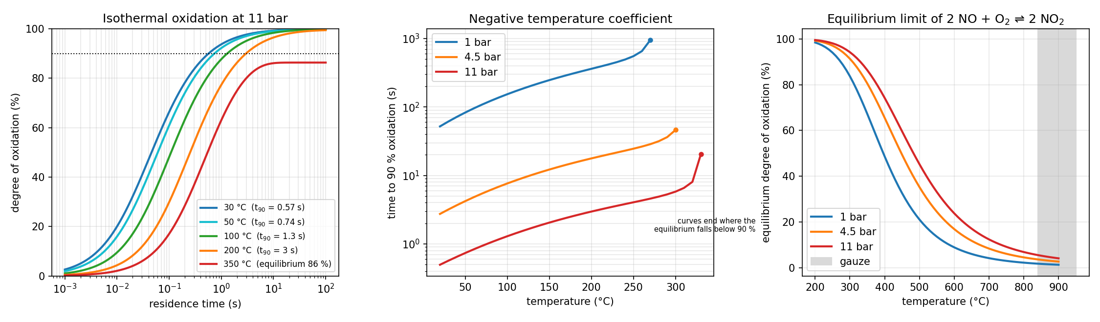
- Pressure. The rate is third order in partial pressures while the amount to be oxidised is first order, so the time falls roughly with the square of the pressure: 61 s at 1 bar, 3.2 s at 4.5 bar and 0.57 s at 11 bar at 30 °C. Oxidation space, and with it the absorption tower, shrinks dramatically with pressure. This is the main reason for high-pressure absorption (Thiemann et al., 2000, Secs. 1.3 and 1.3.4.1).
- Temperature. Cold gas oxidises faster: the time to 90 % grows sixfold from 30 to 200 °C at every pressure. Above about 300 °C a second effect appears, since the equilibrium itself no longer allows 90 % (right panel). At the gauze, the equilibrium degree of oxidation is only 1–4 %, which is why the gas leaving the burner contains practically no NO₂.
- Dimers. At 11 bar and 50 °C, when 90 % of the NO is oxidised, 52 % of the NO₂ is present as N₂O₄. This matters for the next step, because N₂O₄ is the species whose transport to the liquid is considered rate-controlling in the absorption region that makes the acid (Thiemann et al., 2000, Sec. 1.3.2; Hoftyzer & Kwanten, 1972).
The flow sheet states that the gas entering the absorption tower is at least 90 % oxidised (Thiemann et al., 2000, Sec. 1.3.4.1). The model agrees: at 11 bar and 50 °C even fresh NO needs only 0.74 s, and the real gas arrives partly oxidised from the upstream equipment.
"""
Nitric acid — gas-phase oxidation of NO to NO2 (isothermal)
bdrworks.org · Handbook · Nitric acid, worked model 2

    2 NO + O2 -> 2 NO2          third-order, negative temperature coefficient
    2 NO2 <=> N2O4              fast equilibrium
    NO + NO2 <=> N2O3           fast equilibrium

Rate per unit gas volume (O2 consumed), p in atm, r in kmol/(m3 s):
    r = kp/(R T) * (pNO^2 pO2 - pNO2^2 / K_ox),   log10 kp = 652.1/T - 1.0366
The reverse term makes the rate vanish at equilibrium; K_ox comes from NASA polynomials.
A gas parcel of 1 kmol (feed basis) is followed in time at constant T and P:
    d(xi)/dt = kp * n_tot * (pNO^2 pO2 - pNO2^2/K_ox) / P      xi = kmol O2 reacted
Degree of oxidation: alpha = 2 xi / n_NO,0 (N2O4 and N2O3 do not change it).

Run:  python hno3_oxidation.py      (needs numpy, scipy, matplotlib)
"""
import numpy as np
from scipy.integrate import solve_ivp
from scipy.optimize import brentq
import matplotlib.pyplot as plt

RG = 8.314                       # J/(mol K)
ATM = 1.01325                    # bar per atm

# NASA 7-coefficient polynomials (GRI-Mech 3.0): NO, O2, NO2; [T < 1000 K], [T > 1000 K]
NASA_LO = np.array([
    [4.21847630e+00, -4.63897600e-03, 1.10410220e-05, -9.33613540e-09, 2.80357700e-12, 9.84462300e+03, 2.28084640e+00],   # NO
    [3.78245636e+00, -2.99673416e-03, 9.84730201e-06, -9.68129509e-09, 3.24372837e-12, -1.06394356e+03, 3.65767573e+00],  # O2
    [3.94403120e+00, -1.58542900e-03, 1.66578120e-05, -2.04754260e-08, 7.83505640e-12, 2.89661790e+03, 6.31199170e+00],   # NO2
])
NASA_HI = np.array([
    [3.26060560e+00, 1.19110430e-03, -4.29170480e-07, 6.94576690e-11, -4.03360990e-15, 9.92097460e+03, 6.36930270e+00],   # NO
    [3.28253784e+00, 1.48308754e-03, -7.57966669e-07, 2.09470555e-10, -2.16717794e-14, -1.08845772e+03, 5.45323129e+00],  # O2
    [4.88475420e+00, 2.17239560e-03, -8.28069060e-07, 1.57475100e-10, -1.05108950e-14, 2.31649830e+03, -1.17416950e-01],  # NO2
])


def g_RT(T):
    """Dimensionless standard Gibbs energies G/(RT) at 1 bar."""
    a = NASA_LO if T < 1000.0 else NASA_HI
    h = a[:, 0] + a[:, 1]*T/2 + a[:, 2]*T**2/3 + a[:, 3]*T**3/4 + a[:, 4]*T**4/5 + a[:, 5]/T
    s = a[:, 0]*np.log(T) + a[:, 1]*T + a[:, 2]*T**2/2 + a[:, 3]*T**3/3 + a[:, 4]*T**4/4 + a[:, 6]
    return h - s


def K_ox(T):
    """2 NO + O2 = 2 NO2, K = pNO2^2/(pNO^2 pO2) in 1/atm."""
    g = g_RT(T)
    return np.exp(-(2*g[2] - 2*g[0] - g[1])) * ATM


def kp(T):
    return 10.0**(652.1/T - 1.0366)                  # atm^-2 s^-1


def K4(T):
    return 0.698e-9*np.exp(6866.0/T)                 # N2O4/NO2^2, 1/atm


def K3(T):
    return 65.3e-9*np.exp(4740.0/T)                  # N2O3/(NO NO2), 1/atm


def speciate(NOt, NO2t, n_rest, T, P):
    """Free NO, NO2, N2O4, N2O3 (kmol) from the NO and NO2 totals; P in atm."""
    k4, k3 = K4(T)*P, K3(T)*P
    ntot = n_rest + NOt + NO2t
    for _ in range(50):                               # fixed point on the total moles
        def f(b):
            a = NOt/(1.0 + k3*b/ntot)
            return b + 2.0*k4*b*b/ntot + k3*a*b/ntot - NO2t
        b = brentq(f, 0.0, NO2t) if NO2t > 0 else 0.0
        a = NOt/(1.0 + k3*b/ntot)
        c, d = k4*b*b/ntot, k3*a*b/ntot
        new = n_rest + a + b + c + d
        if abs(new - ntot) < 1e-13:
            break
        ntot = new
    return a, b, c, d, new


def rhs(t, y, T, P, n0):
    xi = y[0]
    NOt, O2, NO2t = n0[0] - 2*xi, n0[1] - xi, 2*xi
    a, b, c, d, nt = speciate(max(NOt, 0.0), NO2t, n0[2] + O2, T, P)
    pNO, pO2, pNO2 = a/nt*P, O2/nt*P, b/nt*P
    return [kp(T)*nt*(pNO**2*pO2 - pNO2**2/K_ox(T))/P]


def oxidise(T, P_bar, n0, t_end=1e4):
    P = P_bar/ATM
    stop = lambda t, y, *args: 2*y[0]/n0[0] - 0.9
    stop.terminal = False
    sol = solve_ivp(rhs, (0, t_end), [0.0], args=(T, P, n0), method="LSODA",
                    rtol=1e-8, atol=1e-12, dense_output=True, events=stop)
    t90 = sol.t_events[0][0] if sol.t_events[0].size else np.nan
    return sol, t90


def alpha_eq(T, P_bar, n0):
    """Equilibrium degree of oxidation (monomers only; dimers are negligible when it matters)."""
    P = P_bar/ATM
    def f(al):
        xi = al*n0[0]/2
        n = np.array([n0[0] - 2*xi, n0[1] - xi, 2*xi]); nt = n.sum() + n0[2]
        p = n/nt*P
        return p[2]**2 - K_ox(T)*p[0]**2*p[1]
    return brentq(f, 1e-12, 1 - 1e-12)


def t_analytic(T, P_bar, n0, x):
    """Closed-form isothermal residence time for -dpNO/dt = 2 kp pNO^2 pO2 at constant total moles
    (no reverse reaction, no dimers, no volume contraction)."""
    P = P_bar/ATM
    a, b, k = n0[0]*P, n0[1]*P, 2*kp(T)
    m = 2*b - a
    return 2/(k*m)*(x/(a*(1 - x)) - np.log((2*b - a*x)/(2*b*(1 - x)))/m)


def nitrous_gas(y_nh3=0.10, S=0.965, secondary=0.14):
    """Dry gas after the burner plus secondary air, per kmol (water condensed out).
    secondary = share of the total air sent to the bleacher and added before absorption."""
    prim = 1.0 - y_nh3
    sec = prim*secondary/(1.0 - secondary)
    NO = y_nh3*S
    O2 = 0.2095*(prim + sec) - y_nh3*(1.25*S + 0.75*(1 - S))
    N2 = 0.7905*(prim + sec) + 0.5*y_nh3*(1 - S)
    n = np.array([NO, O2, N2])
    return n/n.sum()


if __name__ == "__main__":
    n0 = nitrous_gas()
    print("dry nitrous gas: NO %.2f %%, O2 %.2f %%, N2 %.2f %%" % tuple(100*n0))
    fig, ax = plt.subplots(1, 3, figsize=(15, 4.4))
    for Tc, c in [(30, "tab:blue"), (50, "tab:cyan"), (100, "tab:green"), (200, "tab:orange"), (350, "tab:red")]:
        sol, t90 = oxidise(Tc + 273.15, 11.0, n0, 100.0)
        t = np.logspace(-3, 2, 300)
        lab = f"t$_{{90}}$ = {t90:.2g} s" if np.isfinite(t90) else f"equilibrium {100*alpha_eq(Tc + 273.15, 11.0, n0):.0f} %"
        ax[0].semilogx(t, 100*2*sol.sol(t)[0]/n0[0], lw=2, color=c, label=f"{Tc} °C  ({lab})")
    ax[0].axhline(90, color="k", ls=":", lw=1)
    ax[0].set(xlabel="residence time (s)", ylabel="degree of oxidation (%)", title="Isothermal oxidation at 11 bar", ylim=(0, 100))
    ax[0].legend(fontsize=8); ax[0].grid(alpha=0.3, which="both")

    Ts = np.arange(20, 401, 10)
    for P, c in [(1.0, "tab:blue"), (4.5, "tab:orange"), (11.0, "tab:red")]:
        t90 = [oxidise(Tc + 273.15, P, n0)[1] for Tc in Ts]
        ax[1].semilogy(Ts, t90, lw=2, color=c, label=f"{P:g} bar")
        k = np.where(np.isfinite(t90))[0][-1]
        ax[1].plot(Ts[k], t90[k], "o", color=c, ms=4)
    ax[1].text(395, 1.5, "curves end where the\nequilibrium falls below 90 %", fontsize=7, ha="right")
    ax[1].set(xlabel="temperature (°C)", ylabel="time to 90 % oxidation (s)", title="Negative temperature coefficient")
    ax[1].legend(); ax[1].grid(alpha=0.3, which="both")

    Te = np.arange(200, 901, 10)
    for P, c in [(1.0, "tab:blue"), (4.5, "tab:orange"), (11.0, "tab:red")]:
        ax[2].plot(Te, [100*alpha_eq(Tc + 273.15, P, n0) for Tc in Te], lw=2, color=c, label=f"{P:g} bar")
    ax[2].axvspan(840, 950, color="0.85", zorder=0, label="gauze")
    ax[2].set(xlabel="temperature (°C)", ylabel="equilibrium degree of oxidation (%)", title="Equilibrium limit of 2 NO + O$_2$ ⇌ 2 NO$_2$")
    ax[2].legend(); ax[2].grid(alpha=0.3)
    fig.tight_layout(); fig.savefig("hno3_oxidation.png", dpi=150)

    print(f"K_ox: 298 K {K_ox(298.15):.3e}, 600 K {K_ox(600):.3e}, 900 K {K_ox(900):.3e} 1/atm")
    print(f"kp: 298 K {kp(298.15):.2f}, 623 K {kp(623.15):.3f} atm^-2 s^-1;  K4(323 K) = {K4(323.15):.3f}, K3(323 K) = {K3(323.15):.3f} 1/atm")
    for P in [1.0, 4.5, 11.0]:
        row = [oxidise(Tc + 273.15, P, n0)[1] for Tc in [30, 50, 100, 200]]
        print(f"{P:5.1f} bar: t90 = " + ", ".join(f"{t:.3g} s" for t in row) + "  (30, 50, 100, 200 °C)")
    for P in [1.0, 4.5, 11.0]:
        print(f"{P:5.1f} bar, 30 °C: closed-form t90 = {t_analytic(303.15, P, n0, 0.9):.3g} s (constant moles, no dimers)")
    for P in [1.0, 4.5, 11.0]:
        print(f"{P:5.1f} bar: equilibrium oxidation 400 °C {100*alpha_eq(673.15, P, n0):.1f} %, 600 °C {100*alpha_eq(873.15, P, n0):.1f} %, 890 °C {100*alpha_eq(1163.15, P, n0):.2f} %")
    a, b, c, d, nt = speciate(0.1*n0[0], 0.9*n0[0], n0[1] - 0.45*n0[0] + n0[2], 323.15, 11.0/ATM)
    print(f"11 bar, 50 °C, 90 % oxidised: NO {a:.4f}, NO2 {b:.4f}, N2O4 {c:.4f}, N2O3 {d:.4f} kmol; N2O4 carries {100*2*c/(0.9*n0[0]):.0f} % of the NO2")
    plt.show()
function hno3_oxidation()
% Nitric acid - isothermal gas-phase oxidation 2 NO + O2 -> 2 NO2
% bdrworks.org - Handbook - Nitric acid, worked model 2
%   d(xi)/dt = kp*n_tot*(pNO^2*pO2 - pNO2^2/K_ox)/P ,  log10 kp = 652.1/T - 1.0366  (atm, s)
%   2 NO2 <=> N2O4 and NO + NO2 <=> N2O3 are fast equilibria
% Save as hno3_oxidation.m and run:  hno3_oxidation      (MATLAB or GNU Octave)

n0 = nitrous_gas(0.10, 0.965, 0.14);
fprintf('dry nitrous gas: NO %.2f %%, O2 %.2f %%, N2 %.2f %%\n', 100*n0);
figure('Position',[60 100 1300 380]);

subplot(1,3,1);
t = logspace(-3, 2, 200);
for Tc = [30 50 100 200 350]
    [ts, xi] = oxidise(Tc + 273.15, 11, n0, 100);
    semilogx(t, 100*2*interp1(ts, xi, t)/n0(1), 'LineWidth', 2); hold on;
end
semilogx([1e-3 1e2], [90 90], 'k:');
xlabel('residence time (s)'); ylabel('degree of oxidation (%)'); title('Isothermal oxidation at 11 bar');
legend('30 \circC','50 \circC','100 \circC','200 \circC','350 \circC','Location','northwest'); grid on;

subplot(1,3,2);
Ts = 20:20:400;
for P = [1 4.5 11]
    t90 = arrayfun(@(Tc) time90(Tc + 273.15, P, n0), Ts);
    semilogy(Ts, t90, 'LineWidth', 2); hold on;
end
xlabel('temperature (\circC)'); ylabel('time to 90 % oxidation (s)'); title('Negative temperature coefficient');
legend('1 bar','4.5 bar','11 bar'); grid on;

subplot(1,3,3);
Te = 200:10:900;
for P = [1 4.5 11]
    plot(Te, 100*arrayfun(@(Tc) alpha_eq(Tc + 273.15, P, n0), Te), 'LineWidth', 2); hold on;
end
xlabel('temperature (\circC)'); ylabel('equilibrium degree of oxidation (%)'); title('Equilibrium limit');
legend('1 bar','4.5 bar','11 bar'); grid on;

fprintf('K_ox(298 K) = %.3e, K_ox(600 K) = %.3e 1/atm;  kp(298 K) = %.2f atm^-2 s^-1\n', K_ox(298.15), K_ox(600), kp(298.15));
for P = [1 4.5 11]
    fprintf('%5.1f bar: t90 = %.3g, %.3g, %.3g, %.3g s  (30, 50, 100, 200 C)\n', P, ...
            time90(303.15, P, n0), time90(323.15, P, n0), time90(373.15, P, n0), time90(473.15, P, n0));
end
for P = [1 4.5 11]
    fprintf('%5.1f bar, 30 C: closed-form t90 = %.3g s (constant moles, no dimers)\n', P, t_analytic(303.15, P, n0, 0.9));
end
for P = [1 4.5 11]
    fprintf('%5.1f bar: equilibrium oxidation 400 C %.1f %%, 600 C %.1f %%, 890 C %.2f %%\n', P, ...
            100*alpha_eq(673.15, P, n0), 100*alpha_eq(873.15, P, n0), 100*alpha_eq(1163.15, P, n0));
end
[a, b, c, d] = speciate(0.1*n0(1), 0.9*n0(1), n0(2) - 0.45*n0(1) + n0(3), 323.15, 11/1.01325);
fprintf('11 bar, 50 C, 90 %% oxidised: NO %.4f, NO2 %.4f, N2O4 %.4f, N2O3 %.4f; N2O4 carries %.0f %% of the NO2\n', ...
        a, b, c, d, 100*2*c/(0.9*n0(1)));
end

% ---------------------------------------------------------------- model
function n = nitrous_gas(y, S, sec)
% dry gas after the burner plus secondary air (share sec of the total air): NO, O2, N2
prim = 1 - y;  s = prim*sec/(1 - sec);
n = [y*S; 0.2095*(prim + s) - y*(1.25*S + 0.75*(1 - S)); 0.7905*(prim + s) + 0.5*y*(1 - S)];
n = n/sum(n);
end

function [ts, xi] = oxidise(T, Pbar, n0, tend)
P = Pbar/1.01325;
opts = odeset('RelTol', 1e-8, 'AbsTol', 1e-12);
[ts, xi] = ode45(@(t, x) rhs(x, T, P, n0), [0 tend], 0, opts);
end

function t90 = time90(T, Pbar, n0)
% time to 90 % oxidation, NaN if the equilibrium lies below 90 %
if alpha_eq(T, Pbar, n0) <= 0.9, t90 = NaN; return; end
[ts, xi] = oxidise(T, Pbar, n0, 1e4);
al = 2*xi/n0(1);
k = find(al >= 0.9, 1);
t90 = interp1(al(k-1:k), ts(k-1:k), 0.9);
end

function dx = rhs(xi, T, P, n0)
NOt = max(n0(1) - 2*xi, 0);  O2 = n0(2) - xi;  NO2t = 2*xi;
[a, b, ~, ~, nt] = speciate(NOt, NO2t, n0(3) + O2, T, P);
pNO = a/nt*P;  pO2 = O2/nt*P;  pNO2 = b/nt*P;
dx = kp(T)*nt*(pNO^2*pO2 - pNO2^2/K_ox(T))/P;
end

function [a, b, c, d, nt] = speciate(NOt, NO2t, nrest, T, P)
% free NO (a), NO2 (b), N2O4 (c), N2O3 (d) from the totals; P in atm
% outer fixed point on the total moles, inner Newton iteration on the free NO2
k4 = K4(T)*P;  k3 = K3(T)*P;  nt = nrest + NOt + NO2t;  b = NO2t;
for it = 1:50
    for jt = 1:60
        f  = b + 2*k4*b^2/nt + k3*NOt*b/(nt + k3*b) - NO2t;
        df = 1 + 4*k4*b/nt + k3*NOt*nt/(nt + k3*b)^2;
        bn = min(max(b - f/df, 0), NO2t);
        if abs(bn - b) <= 1e-15*max(NO2t, 1e-30), b = bn; break; end
        b = bn;
    end
    a = NOt/(1 + k3*b/nt);  c = k4*b^2/nt;  d = k3*a*b/nt;
    new = nrest + a + b + c + d;
    if abs(new - nt) < 1e-13, nt = new; break; end
    nt = new;
end
end

function t = t_analytic(T, Pbar, n0, x)
% closed-form isothermal time for -dpNO/dt = 2 kp pNO^2 pO2 at constant total moles
P = Pbar/1.01325;  a = n0(1)*P;  b = n0(2)*P;  k = 2*kp(T);  m = 2*b - a;
t = 2/(k*m)*(x/(a*(1 - x)) - log((2*b - a*x)/(2*b*(1 - x)))/m);
end

function al = alpha_eq(T, Pbar, n0)
P = Pbar/1.01325;
f = @(al) resid(al, T, P, n0);
al = fzero(f, [1e-12 1 - 1e-12]);
end

function r = resid(al, T, P, n0)
xi = al*n0(1)/2;
n = [n0(1) - 2*xi; n0(2) - xi; 2*xi];  nt = sum(n) + n0(3);
p = n/nt*P;
r = p(3)^2 - K_ox(T)*p(1)^2*p(2);
end

function k = kp(T),  k = 10^(652.1/T - 1.0366);  end        % atm^-2 s^-1
function K = K4(T),  K = 0.698e-9*exp(6866/T);   end        % N2O4/NO2^2, 1/atm
function K = K3(T),  K = 65.3e-9*exp(4740/T);    end        % N2O3/(NO NO2), 1/atm

function K = K_ox(T)
% 2 NO + O2 = 2 NO2 from NASA polynomials (GRI-Mech 3.0): NO, O2, NO2; 1/atm
lo = [4.21847630e+00 -4.63897600e-03 1.10410220e-05 -9.33613540e-09 2.80357700e-12 9.84462300e+03 2.28084640e+00
      3.78245636e+00 -2.99673416e-03 9.84730201e-06 -9.68129509e-09 3.24372837e-12 -1.06394356e+03 3.65767573e+00
      3.94403120e+00 -1.58542900e-03 1.66578120e-05 -2.04754260e-08 7.83505640e-12 2.89661790e+03 6.31199170e+00];
hi = [3.26060560e+00 1.19110430e-03 -4.29170480e-07 6.94576690e-11 -4.03360990e-15 9.92097460e+03 6.36930270e+00
      3.28253784e+00 1.48308754e-03 -7.57966669e-07 2.09470555e-10 -2.16717794e-14 -1.08845772e+03 5.45323129e+00
      4.88475420e+00 2.17239560e-03 -8.28069060e-07 1.57475100e-10 -1.05108950e-14 2.31649830e+03 -1.17416950e-01];
if T < 1000, a = lo; else, a = hi; end
g = a(:,1)*(1 - log(T)) - a(:,2)*T/2 - a(:,3)*T^2/6 - a(:,4)*T^3/12 - a(:,5)*T^4/20 + a(:,6)/T - a(:,7);
K = exp(-(2*g(3) - 2*g(1) - g(2)))*1.01325;
end
6Solution 3 · The nitrous-gas train
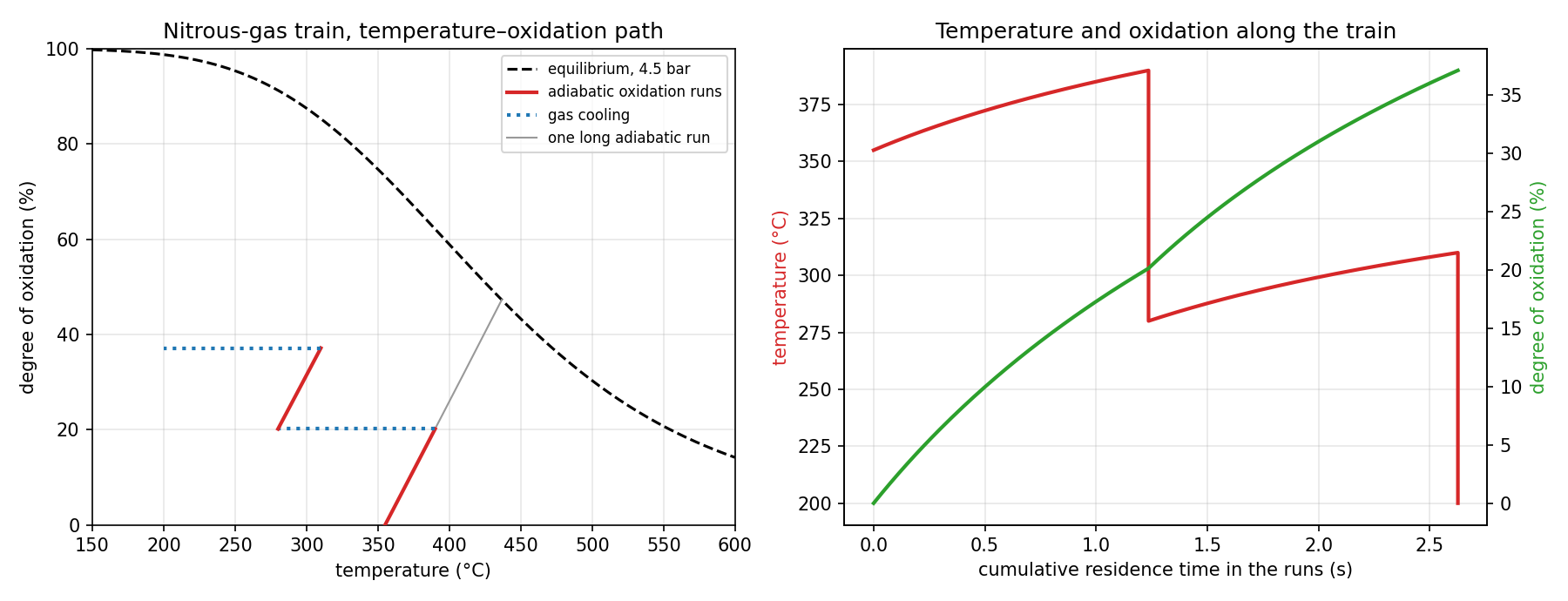
Between the waste-heat boiler and the cooler–condensers, the gas is still hot and wet (Table in Solution 1) and flows through large pipes and exchangers at about 4.5 bar. The dual-pressure flow sheet gives its temperatures: 355 °C after the boiler, 390 °C after a run of piping for oxidation, 280 °C after tail-gas preheater III, 310 °C after further oxidation and 200 °C after the economizer (Thiemann et al., 2000, Sec. 1.3.4.1 and Fig. 29). The temperature rises in the pipes are the heat of NO oxidation. Treating each run as an adiabatic plug-flow section, Eq. 7 is joined by an energy balance:
The second line is the same estimate as the layer-by-layer temperature rise that Ullmann gives for adiabatic oxidation spaces (Thiemann et al., 2000, Sec. 1.3.2, Eq. 46): complete oxidation of this gas would heat it by about 174 K. N₂O₄ and N₂O₃ are left out here; above 200 °C at 4.5 bar they hold less than 0.1 % of the NO₂. Each run is integrated until the temperature reaches the value of the flow sheet, with an event function in the ODE solver; the time this takes is the residence time the plant data imply. The exchangers are treated as instantaneous coolers, so the oxidation that also occurs inside them is lumped into the runs.
| Section (1000 t/d HNO₃) | T in → out | Residence time | Oxidation | Duty |
|---|---|---|---|---|
| Oxidation run 1 | 355 → 390 °C | 1.24 s | 0 → 20.2 % | adiabatic |
| Tail-gas preheater III | 390 → 280 °C | — | 20.2 % | 6.7 MW |
| Oxidation run 2 | 280 → 310 °C | 1.39 s | 20.2 → 37.1 % | adiabatic |
| Economizer | 310 → 200 °C | — | 37.1 % | 6.6 MW |
The plant capacity is set at 1000 t/d of HNO₃ with the dual-pressure ammonia consumption of 279 kg per tonne of acid (Thiemann et al., 2000, Table 5), which gives 6826 kmol/h of ammonia–air mixture and about 24 m³/s of nitrous gas in the first run. The implied residence times of 1.2–1.4 s correspond to 25–30 m of pipe at 20 m/s, a plausible length for the large-bore piping between the boiler and the exchangers, and a velocity well below the rule-of-thumb limit of about 60 m/s for gas lines (Walas, 1990, Ch. 1, rules of thumb). The model and the flow sheet are consistent.
The temperature–oxidation diagram has the same structure as that of a multi-bed adiabatic converter with interstage cooling. Each adiabatic run moves along a straight line, up and to the right, towards the equilibrium curve; each cooler moves the gas back to the left at constant composition. A single long adiabatic run from 355 °C would stall at 47 % oxidation and 437 °C, on the equilibrium curve, however long the pipe. The difference is in the motive: in an exothermic synthesis converter the beds are cooled to escape the equilibrium, while here the kinetics alone would ask for the coldest possible gas. The plant instead takes the heat out in steps at 200–390 °C, where it preheats the tail gas for the expansion turbine and the boiler feed water, and completes the oxidation later, cold and at high pressure (Thiemann et al., 2000, Sec. 1.3.4.1).
"""
Nitric acid — NO oxidation in the nitrous-gas train of a dual-pressure plant
bdrworks.org · Handbook · Nitric acid, worked model 3

The gas leaving the waste-heat boiler oxidises in adiabatic runs of piping and is cooled in
the tail-gas preheater and the economizer (flow sheet of the dual-pressure process):
    WHB outlet 355 °C -> pipe run -> 390 °C -> tail-gas preheater III -> 280 °C
                      -> pipe run -> 310 °C -> economizer -> 200 °C
Each run is an adiabatic plug-flow section followed in time (Lagrangian gas parcel):
    d(xi)/dt = kp * n_tot * (pNO^2 pO2 - pNO2^2/K_ox) / P                 (xi = kmol O2 reacted)
    dT/dt    = -dH_ox(T) * d(xi)/dt / sum(n_i cp_i)                        (adiabatic)
An event stops each run at the outlet temperature of the flow sheet; the time it takes is
the residence time the flow sheet implies. Heat exchangers are treated as instantaneous
coolers (oxidation inside them is lumped into the runs). N2O4 and N2O3 are negligible above
~170 °C at 4.5 bar and are left out.

Run:  python hno3_train.py      (needs numpy, scipy, matplotlib)
"""
import numpy as np
from scipy.integrate import solve_ivp
from scipy.optimize import brentq
import matplotlib.pyplot as plt

RG = 8.314                                 # J/(mol K)
ATM = 1.01325                              # bar per atm
SP = ["NO", "O2", "NO2", "H2O", "N2"]
NU = np.array([-2.0, -1.0, 2.0, 0.0, 0.0])  # 2 NO + O2 -> 2 NO2

# NASA 7-coefficient polynomials (GRI-Mech 3.0), 200-1000 K
NASA = np.array([
    [4.21847630e+00, -4.63897600e-03, 1.10410220e-05, -9.33613540e-09, 2.80357700e-12, 9.84462300e+03, 2.28084640e+00],   # NO
    [3.78245636e+00, -2.99673416e-03, 9.84730201e-06, -9.68129509e-09, 3.24372837e-12, -1.06394356e+03, 3.65767573e+00],  # O2
    [3.94403120e+00, -1.58542900e-03, 1.66578120e-05, -2.04754260e-08, 7.83505640e-12, 2.89661790e+03, 6.31199170e+00],   # NO2
    [4.19864056e+00, -2.03643410e-03, 6.52040211e-06, -5.48797062e-09, 1.77197817e-12, -3.02937267e+04, -8.49032208e-01],  # H2O
    [3.29867700e+00, 1.40824040e-03, -3.96322200e-06, 5.64151500e-09, -2.44485400e-12, -1.02089990e+03, 3.95037200e+00],   # N2
])


def cp(T):
    a = NASA
    return RG*(a[:, 0] + a[:, 1]*T + a[:, 2]*T**2 + a[:, 3]*T**3 + a[:, 4]*T**4)


def h(T):
    a = NASA
    return RG*T*(a[:, 0] + a[:, 1]*T/2 + a[:, 2]*T**2/3 + a[:, 3]*T**3/4 + a[:, 4]*T**4/5 + a[:, 5]/T)


def g_RT(T):
    a = NASA
    return (a[:, 0]*(1 - np.log(T)) - a[:, 1]*T/2 - a[:, 2]*T**2/6 - a[:, 3]*T**3/12 - a[:, 4]*T**4/20
            + a[:, 5]/T - a[:, 6])


def K_ox(T):
    """pNO2^2/(pNO^2 pO2), 1/atm."""
    return np.exp(-(NU @ g_RT(T))) * ATM


def kp(T):
    return 10.0**(652.1/T - 1.0366)          # atm^-2 s^-1


def burner_gas(y_nh3=0.10, S=0.965):
    """Gas after the gauze per kmol of NH3-air mixture (see hno3_burner.py)."""
    air = 1.0 - y_nh3
    NO = y_nh3*S
    O2 = 0.2095*air - y_nh3*(1.25*S + 0.75*(1 - S))
    N2 = 0.7905*air + 0.5*y_nh3*(1 - S)
    return np.array([NO, O2, 0.0, 1.5*y_nh3, N2])


def rate(n, T, P):
    """d(xi)/dt for a parcel with moles n at T (K) and P (atm)."""
    nt = n.sum()
    p = n/nt*P
    return kp(T)*nt*(p[0]**2*p[1] - p[2]**2/K_ox(T))/P


def run(n_in, T_in, P, T_out=None, t_max=60.0):
    """Adiabatic run from (n_in, T_in); stops when T reaches T_out (or at t_max)."""
    def rhs(t, y):
        n = n_in + NU*y[0]
        r = rate(n, y[1], P)
        return [r, -(NU @ h(y[1]))*r/(n @ cp(y[1]))]
    ev = (lambda t, y: y[1] - T_out) if T_out else None
    if ev:
        ev.terminal = True
    sol = solve_ivp(rhs, (0, t_max), [0.0, T_in], method="LSODA", rtol=1e-9, atol=1e-12,
                    events=ev, dense_output=True, max_step=0.05)
    return sol


def alpha_eq(T, n_in, P):
    def f(al):
        n = n_in + NU*al*n_in[0]/2
        p = n/n.sum()*P
        return p[2]**2 - K_ox(T)*p[0]**2*p[1]
    return brentq(f, 1e-12, 1 - 1e-12)


def duty(n, T1, T2):
    """Heat removed when cooling n from T1 to T2, J per kmol-basis mol."""
    return n @ (h(T1) - h(T2))


if __name__ == "__main__":
    P = 4.5/ATM                              # atm, after the burner and the waste-heat boiler
    n0 = burner_gas()                        # per mol NH3-air mixture
    N_mix = 6826/3600.0                      # kmol/s of mixture: 1000 t/d HNO3 at 279 kg NH3/t, 10 % NH3
    steps = [("run 1", 355, 390), ("tail-gas preheater III", 390, 280), ("run 2", 280, 310), ("economizer", 310, 200)]
    n, T, t_tot = n0.copy(), 355 + 273.15, 0.0
    tr, Tr, ar, path = [], [], [], []
    print(f"gas after burner: " + ", ".join(f"{s} {100*x:.2f} %" for s, x in zip(SP, n0/n0.sum())))
    for name, Ti, To in steps:
        if name.startswith("run"):
            sol = run(n, T, P, To + 273.15)
            tau = sol.t[-1]
            ts = np.linspace(0, tau, 100)
            xi = sol.sol(ts)[0]; Ts = sol.sol(ts)[1]
            tr += list(t_tot + ts); Tr += list(Ts - 273.15); ar += list(100*(n[2] + 2*xi)/n0[0])
            path.append((np.array(ar[-100:]), Ts - 273.15, "-"))
            a_in = 100*n[2]/n0[0]
            n = n + NU*xi[-1]; T = Ts[-1]; t_tot += tau
            V = N_mix*n.sum()*1e3*RG*T/(P*101325)
            print(f"{name}: {Ti} -> {To} °C in {tau:.2f} s; oxidation {a_in:.1f} -> {100*n[2]/n0[0]:.1f} %; "
                  f"{V:.1f} m3/s, {20*tau:.0f} m of pipe at 20 m/s")
        else:
            Q = duty(n, T, To + 273.15)*N_mix*1e3/1e6
            a = 100*n[2]/n0[0]
            path.append((np.array([a, a]), np.array([T - 273.15, To]), ":"))
            T = To + 273.15
            tr.append(t_tot); Tr.append(To); ar.append(a)
            print(f"{name}: {Ti} -> {To} °C, duty {Q:.1f} MW at {a:.1f} % oxidation")
    # a single long adiabatic run from 355 °C for comparison
    long = run(n0, 355 + 273.15, P, None, 60.0)
    tl = np.linspace(0, 60, 400); xl, Tl = long.sol(tl)
    print(f"one long adiabatic run: after 60 s {100*2*xl[-1]/n0[0]:.1f} % at {Tl[-1]-273.15:.0f} °C "
          f"(equilibrium at that T: {100*alpha_eq(Tl[-1], n0, P):.1f} %)")
    dT = -(NU @ h(630))*n0[0]/2/(n0 @ cp(630))
    print(f"adiabatic temperature rise for complete oxidation: {dT:.0f} K")

    fig, ax = plt.subplots(1, 2, figsize=(12, 4.6))
    Te = np.linspace(150, 600, 200)
    ax[0].plot(Te, [100*alpha_eq(t + 273.15, n0, P) for t in Te], "k--", lw=1.5, label="equilibrium, 4.5 bar")
    for i, (a, Tt, ls) in enumerate(path):
        ax[0].plot(Tt, a, ls, color="tab:red" if ls == "-" else "tab:blue", lw=2, zorder=3,
                   label=("adiabatic oxidation runs" if i == 0 else "gas cooling" if i == 1 else None))
    ax[0].plot(Tl - 273.15, 100*2*xl/n0[0], color="0.6", lw=1, zorder=2, label="one long adiabatic run")
    ax[0].set(xlabel="temperature (°C)", ylabel="degree of oxidation (%)", xlim=(150, 600), ylim=(0, 100),
              title="Nitrous-gas train, temperature–oxidation path")
    ax[0].legend(fontsize=8); ax[0].grid(alpha=0.3)
    ax[1].plot(tr, Tr, color="tab:red", lw=2); ax[1].set_ylabel("temperature (°C)", color="tab:red")
    b = ax[1].twinx(); b.plot(tr, ar, color="tab:green", lw=2); b.set_ylabel("degree of oxidation (%)", color="tab:green")
    ax[1].set(xlabel="cumulative residence time in the runs (s)", title="Temperature and oxidation along the train")
    ax[1].grid(alpha=0.3)
    fig.tight_layout(); fig.savefig("hno3_train.png", dpi=150)
    plt.show()
function hno3_train()
% Nitric acid - NO oxidation in the nitrous-gas train of a dual-pressure plant
% bdrworks.org - Handbook - Nitric acid, worked model 3
%   adiabatic runs:  d(xi)/dt = kp*n_tot*(pNO^2*pO2 - pNO2^2/K_ox)/P
%                    dT/dt    = -dH_ox(T)*d(xi)/dt / sum(n_i cp_i)
%   each run stops at the outlet temperature of the flow sheet (event); coolers are instantaneous
% Save as hno3_train.m and run:  hno3_train      (MATLAB or GNU Octave)

P = 4.5/1.01325;                     % atm
nu = [-2; -1; 2; 0; 0];              % NO, O2, NO2, H2O, N2
n0 = burner_gas(0.10, 0.965);
Nmix = 6826/3600;                    % kmol/s of NH3-air mixture (1000 t/d HNO3)
fprintf('gas after burner: NO %.2f %%, O2 %.2f %%, H2O %.2f %%, N2 %.2f %%\n', 100*n0([1 2 4 5])/sum(n0));
steps = {'run 1', 355, 390; 'tail-gas preheater III', 390, 280; 'run 2', 280, 310; 'economizer', 310, 200};
n = n0;  T = 355 + 273.15;  ttot = 0;
figure('Position',[100 100 1100 400]);
subplot(1,2,1); hold on;
Te = linspace(150, 600, 120);
plot(Te, 100*arrayfun(@(t) alpha_eq(t + 273.15, n0, P, nu), Te), 'k--');
for k = 1:size(steps, 1)
    To = steps{k,3} + 273.15;
    if strncmp(steps{k,1}, 'run', 3)
        ev = @(t, u) event_T(u, To);
        opts = odeset('RelTol', 1e-9, 'AbsTol', 1e-12, 'Events', ev, 'MaxStep', 0.05);
        [ts, u] = ode45(@(t, u) rhs(u, n, P, nu), [0 60], [0; T], opts);
        a_in = 100*n(3)/n0(1);
        al = 100*(n(3) + 2*u(:,1))/n0(1);
        subplot(1,2,1); plot(u(:,2) - 273.15, al, 'r', 'LineWidth', 2);
        subplot(1,2,2); plot(ttot + ts, u(:,2) - 273.15, 'r', 'LineWidth', 2); hold on;
        n = n + nu*u(end,1);  T = u(end,2);  ttot = ttot + ts(end);
        fprintf('%s: %d -> %d C in %.2f s; oxidation %.1f -> %.1f %%\n', steps{k,1}, steps{k,2}, steps{k,3}, ts(end), a_in, 100*n(3)/n0(1));
    else
        Q = n'*(h_all(T) - h_all(To))*Nmix*1e3/1e6;
        a = 100*n(3)/n0(1);
        subplot(1,2,1); plot([T To] - 273.15, [a a], 'b:', 'LineWidth', 2);
        T = To;
        fprintf('%s: %d -> %d C, duty %.1f MW at %.1f %% oxidation\n', steps{k,1}, steps{k,2}, steps{k,3}, Q, a);
    end
end
opts = odeset('RelTol', 1e-9, 'AbsTol', 1e-12, 'MaxStep', 0.05);
[tl, ul] = ode45(@(t, u) rhs(u, n0, P, nu), [0 60], [0; 355 + 273.15], opts);
fprintf('one long adiabatic run: after 60 s %.1f %% at %.0f C\n', 100*2*ul(end,1)/n0(1), ul(end,2) - 273.15);
subplot(1,2,1); plot(ul(:,2) - 273.15, 100*2*ul(:,1)/n0(1), 'Color', [0.6 0.6 0.6]);
xlabel('temperature (\circC)'); ylabel('degree of oxidation (%)'); xlim([150 600]); ylim([0 100]); grid on;
title('Temperature-oxidation path');
subplot(1,2,2); xlabel('cumulative residence time in the runs (s)'); ylabel('temperature (\circC)'); grid on;
end

function [value, isterminal, direction] = event_T(u, To)
value = u(2) - To;  isterminal = 1;  direction = 0;
end

function du = rhs(u, nin, P, nu)
n = nin + nu*u(1);  T = u(2);
r = rate(n, T, P);
du = [r; -(nu'*h_all(T))*r/(n'*cp_all(T))];
end

function r = rate(n, T, P)
nt = sum(n);  p = n/nt*P;
r = kp(T)*nt*(p(1)^2*p(2) - p(3)^2/K_ox(T))/P;
end

function n = burner_gas(y, S)
air = 1 - y;
n = [y*S; 0.2095*air - y*(1.25*S + 0.75*(1 - S)); 0; 1.5*y; 0.7905*air + 0.5*y*(1 - S)];
end

function al = alpha_eq(T, nin, P, nu)
f = @(al) eqres(al, T, nin, P, nu);
al = fzero(f, [1e-12 1 - 1e-12]);
end

function r = eqres(al, T, nin, P, nu)
n = nin + nu*al*nin(1)/2;  p = n/sum(n)*P;
r = p(3)^2 - K_ox(T)*p(1)^2*p(2);
end

function k = kp(T),  k = 10^(652.1/T - 1.0366);  end      % atm^-2 s^-1

% ---------------------------------------------------------------- NASA polynomials (GRI-Mech 3.0), 200-1000 K
function a = nasa()
a = [4.21847630e+00 -4.63897600e-03 1.10410220e-05 -9.33613540e-09 2.80357700e-12 9.84462300e+03 2.28084640e+00    % NO
     3.78245636e+00 -2.99673416e-03 9.84730201e-06 -9.68129509e-09 3.24372837e-12 -1.06394356e+03 3.65767573e+00   % O2
     3.94403120e+00 -1.58542900e-03 1.66578120e-05 -2.04754260e-08 7.83505640e-12 2.89661790e+03 6.31199170e+00    % NO2
     4.19864056e+00 -2.03643410e-03 6.52040211e-06 -5.48797062e-09 1.77197817e-12 -3.02937267e+04 -8.49032208e-01  % H2O
     3.29867700e+00 1.40824040e-03 -3.96322200e-06 5.64151500e-09 -2.44485400e-12 -1.02089990e+03 3.95037200e+00];  % N2
end

function c = cp_all(T)
a = nasa();  c = 8.314*(a(:,1) + a(:,2)*T + a(:,3)*T^2 + a(:,4)*T^3 + a(:,5)*T^4);
end

function hh = h_all(T)
a = nasa();  hh = 8.314*T*(a(:,1) + a(:,2)*T/2 + a(:,3)*T^2/3 + a(:,4)*T^3/4 + a(:,5)*T^4/5 + a(:,6)/T);
end

function K = K_ox(T)
a = nasa();
g = a(:,1)*(1 - log(T)) - a(:,2)*T/2 - a(:,3)*T^2/6 - a(:,4)*T^3/12 - a(:,5)*T^4/20 + a(:,6)/T - a(:,7);
K = exp(-(2*g(3) - 2*g(1) - g(2)))*1.01325;
end
7Model and plant
| Quantity | Model | Plant or literature |
|---|---|---|
| Gauze, 10 % NH₃ at 220 °C | 894 °C | 890 °C (Thiemann et al., 2000, Sec. 1.3.4.1) |
| Gauze, 10.7 % NH₃ at 175 °C | 899 °C | ca. 900 °C (Thiemann et al., 2000, Sec. 1.3.4.1) |
| Average rise per % NH₃ (0 → 10 %, mixture at 200 °C) | 67.8 K | ca. 68 K (Thiemann et al., 2000, Eq. 9) |
| Heat of reaction, Eq. 1 | −902 kJ | −904 kJ (Thiemann et al., 2000, Eq. 4) |
| kp at 25 °C | 14.1 atm⁻²s⁻¹ | 11.8 (Davis & Davis, 2003, Table 1.4.3) |
| Isothermal time to 90 %, 1 bar, 30 °C, constant moles | 65.0 s | 65.0 s, Eq. 8 (Thiemann et al., 2000, Eq. 43) |
| Oxidation run 1, 355 → 390 °C | 1.24 s | 25 m of pipe at 20 m/s |
| Gas entering absorption | 90 % in 0.74 s | ≥ 90 % oxidised (Thiemann et al., 2000, Sec. 1.3.4.1) |
The agreement on temperatures is expected, since both the model and the rule of thumb are energy balances. The agreement on the residence times is a real test of the kinetics, and the model passes it within the uncertainty of the flow-sheet temperatures.
8Try it
The same models, ported to JavaScript and solved with an adaptive Runge–Kutta integrator (Dormand & Prince, 1980), run below. Change the ammonia ratio, the pressure or the temperatures to see how each step responds.
9Going further
- Add the N₂O selectivity to the burner. Ullmann's Eq. 5 releases −1105 kJ per 4 mol NH₃, and N₂O is a strong greenhouse gas that modern plants must abate (Thiemann et al., 2000, Secs. 1.3.1 and 1.4.2).
- Model the waste-heat boiler as a cooled plug-flow section from 890 to 355 °C and see where oxidation starts; the reverse term of Eq. 5 decides it.
- Replace the instantaneous coolers of Solution 3 with exchangers of finite residence time and a U · A per metre, and fit the pipe lengths again.
- Build a plate-to-plate absorption model with the equilibrium method of Ullmann's Eqs. 40 and 41, alternating an absorption stage and an oxidation space between plates (Thiemann et al., 2000, Sec. 1.3.2; Hoftyzer & Kwanten, 1972). The liquid-phase steps, first-order N₂O₄ hydrolysis and HNO₂ decomposition, are given there as Eqs. 20–25 (Andrew & Hanson, 1961).
- Compare the oxidation space as a plug-flow and as a stirred-tank reactor, the two limits Thiemann et al. discuss for bubble-cap and sieve trays (Thiemann et al., 2000, Sec. 1.3.2; Levenspiel, 1999, Ch. 6).
10References
- Andrew, S. P. S., & Hanson, D. (1961). The dynamics of nitrous gas absorption. Chem. Eng. Sci., 14, 105–113.
- Bodenstein, M. (1922). Bildung und Zersetzung der höheren Stickoxyde. Z. Phys. Chem., 100, 68–123.
- Brent, R. P. (1973). Algorithms for Minimization without Derivatives. Prentice-Hall, Englewood Cliffs, NJ.
- Davis, M. E., & Davis, R. J. (2003). Fundamentals of Chemical Reaction Engineering. McGraw-Hill, New York.
- Dormand, J. R., & Prince, P. J. (1980). A family of embedded Runge–Kutta formulae. J. Comput. Appl. Math., 6(1), 19–26.
- Finlayson, B. A., Biegler, L. T., & Grossmann, I. E. (2006). Mathematics in chemical engineering. In Ullmann's Encyclopedia of Industrial Chemistry. Wiley-VCH, Weinheim. doi:10.1002/14356007.b01_01.pub2
- Fogler, H. S. (2016). Elements of Chemical Reaction Engineering (5th ed.). Prentice Hall, Boston.
- Gordon, S., & McBride, B. J. (1994). Computer Program for Calculation of Complex Chemical Equilibrium Compositions and Applications (CEA), Part I: Analysis. NASA Reference Publication 1311, Cleveland, OH.
- Hlavacek, V., Puszynski, J. A., Viljoen, H. J., & Gatica, J. E. (2000). Model reactors and their design equations. In Ullmann's Encyclopedia of Industrial Chemistry. Wiley-VCH, Weinheim. doi:10.1002/14356007.b04_121
- Hoftyzer, P. J., & Kwanten, F. J. G. (1972). Absorption of nitrous gases. In Gas Purification Processes for Air Pollution Control (Nonhebel, G., Ed.). Butterworths, London.
- Levenspiel, O. (1999). Chemical Reaction Engineering (3rd ed.). Wiley, New York.
- Petzold, L. (1983). Automatic selection of methods for solving stiff and nonstiff systems of ordinary differential equations. SIAM J. Sci. Stat. Comput., 4(1), 136–148.
- Shampine, L. F., & Reichelt, M. W. (1997). The MATLAB ODE suite. SIAM J. Sci. Comput., 18(1), 1–22.
- Smith, G. P., Golden, D. M., Frenklach, M., Moriarty, N. W., Eiteneer, B., Goldenberg, M., Bowman, C. T., Hanson, R. K., Song, S., Gardiner, W. C., Lissianski, V. V., & Qin, Z. (1999). GRI-Mech 3.0 (thermodynamic data, NASA polynomials). Gas Research Institute, http://combustion.berkeley.edu/gri-mech/.
- Smith, J. M., Van Ness, H. C., Abbott, M. M., & Swihart, M. T. (2018). Introduction to Chemical Engineering Thermodynamics (8th ed.). McGraw-Hill Education, New York.
- Thiemann, M., Scheibler, E., & Wiegand, K. W. (2000). Nitric acid, nitrous acid, and nitrogen oxides. In Ullmann's Encyclopedia of Industrial Chemistry. Wiley-VCH, Weinheim. doi:10.1002/14356007.a17_293
- Virtanen, P., Gommers, R., Oliphant, T. E., et al. (2020). SciPy 1.0: fundamental algorithms for scientific computing in Python. Nat. Methods, 17, 261–272.
- Walas, S. M. (1990). Chemical Process Equipment: Selection and Design. Butterworth-Heinemann, Boston.
The plant case follows the dual-pressure flow sheet described in Ullmann's Encyclopedia; the capacity, the pipe velocity and the treatment of the exchangers are round-number assumptions for teaching, not data from a specific plant.