1The problem
Steam reforming of natural gas produces most of the world's hydrogen and synthesis gas: the feed of every ammonia and most methanol plants. It is the opposite kind of problem to the two previous models. There the reaction released heat and the difficulty was removing it; here it absorbs a great deal of heat at very high temperature, and the difficulty is supplying it (Rostrup-Nielsen, 1984; Appl, 2000, Sec. 4.5.1.1).
Reforming is strongly endothermic and produces moles. Equilibrium therefore favours high temperature and low pressure (Fiedler et al., 2000, Sec. 5.1). Downstream users need the gas at 25–40 bar, and compressing the product costs more than compressing the feed, so reformers run at high pressure and make up for it with temperatures of 1100–1300 K. The tube material sets the limit: the tubes creep, and their time to rupture depends on wall temperature and internal pressure (Appl, 2000, Sec. 4.5.1.1). The three solutions below show the thermodynamic limit and then the two ways of supplying the heat: through a tube wall from a furnace, or by combustion inside the reactor.
2Process
In a conventional plant the natural gas is first desulphurised over cobalt–molybdenum and zinc oxide catalysts, because nickel is poisoned by sulphur (Appl, 2000, Sec. 4.5.1.1; Fiedler et al., 2000, Sec. 5.1). It is mixed with steam, preheated to about 800 K and passed through hundreds of vertical tubes filled with nickel catalyst (15–25 % NiO on α-alumina, calcium aluminate or magnesium aluminate spinel). A furnace holds 200–400 centrifugally cast tubes, 10–13 m long, with inner diameters of 75–140 mm and walls 11–18 mm thick (Appl, 2000, Sec. 4.5.1.1). The tubes hang in a furnace fired by burners on the roof, the walls or the floor (top-fired, side-fired, terraced-wall or bottom-fired designs) (Appl, 2000, Sec. 4.5.1.1). Most of the fired heat reaches the tubes by radiation, and the rest is recovered in the convection section to preheat feeds and raise steam.
The steam-to-carbon ratio S/C (mol H₂O per mol C) is the main process variable. Excess steam pushes the equilibrium towards conversion and, just as importantly, prevents carbon formation on the nickel. Carbon can form by methane cracking (CH₄ → C + 2H₂) or by the Boudouard reaction (2CO → C + CO₂); it deactivates the catalyst and causes local overheating of the tubes, seen as hot bands (Appl, 2000, Sec. 4.5.1.1; Fiedler et al., 2000, Sec. 5.1; Rostrup-Nielsen, 1984). Modern tubular reformers for natural gas run at S/C ≈ 2.8–3.5 (Appl, 2000, Sec. 4.5.1.1). Autothermal reformers, protected by their combustion zone, run as low as 0.6.
3Kinetics
The standard kinetic model is that of Xu and Froment, derived from a Langmuir–Hinshelwood mechanism on nickel. The three reactions of Eq. 1 share one adsorption term (Xu & Froment, 1989a; Froment et al., 2011, Ch. 11):
with the constants of the original work (k in kmol, kgcat, h, bar; activation energies and heats of adsorption in kJ/mol) (Xu & Froment, 1989a):
| Parameter | Pre-exponential | E or ΔH (kJ/mol) |
|---|---|---|
| k₁ | 4.225 × 10¹⁵ | 240.1 |
| k₂ | 1.955 × 10⁶ | 67.13 |
| k₃ | 1.020 × 10¹⁵ | 243.9 |
| KCO, KH₂, KCH₄ | 8.23 × 10⁻⁵, 6.12 × 10⁻⁹, 6.65 × 10⁻⁴ | −70.65, −82.90, −38.28 |
| KH₂O | 1.77 × 10⁵ | 88.68 |
Industrial reformer pellets are large and the intrinsic reaction is very fast, so only a thin outer shell of each pellet works. The effectiveness factors ηj are of order 0.01–0.1 (Xu & Froment, 1989b). The models here use η = 0.03 for all three reactions, a simplification of a proper pellet diffusion calculation. Even so, the bed stays close to equilibrium along most of the tube. The reformer is limited by heat transfer, not by the catalyst.
Thermodynamic properties come from the NASA seven-coefficient polynomials of the GRI-Mech 3.0 database, which are valid up to 3 500 K (Smith et al., 1999; Gordon & McBride, 1994). That matters for the flame temperatures of Solution 3. The equilibrium constants of Eq. 2 agree with the same database to within about 3 % up to 1 000 K and 7 % at 1 200 K.
4Solution 1 · Equilibrium limit
Before any reactor is designed, equilibrium sets the best possible outcome. Reactions 1 and 2 are independent, and 3 is their sum, so two extents of reaction are found from the two conditions of Eq. 2. The Python code uses fsolve; the MATLAB code has a small damped Newton solver, so no toolbox is needed (Finlayson et al., 2006, Sec. 1.3). The Python results were also checked against a full Gibbs-energy minimisation with Cantera (Goodwin et al., 2023) and agree to within 0.7 percentage points of methane conversion between 800 and 1 300 K and 1–40 bar.
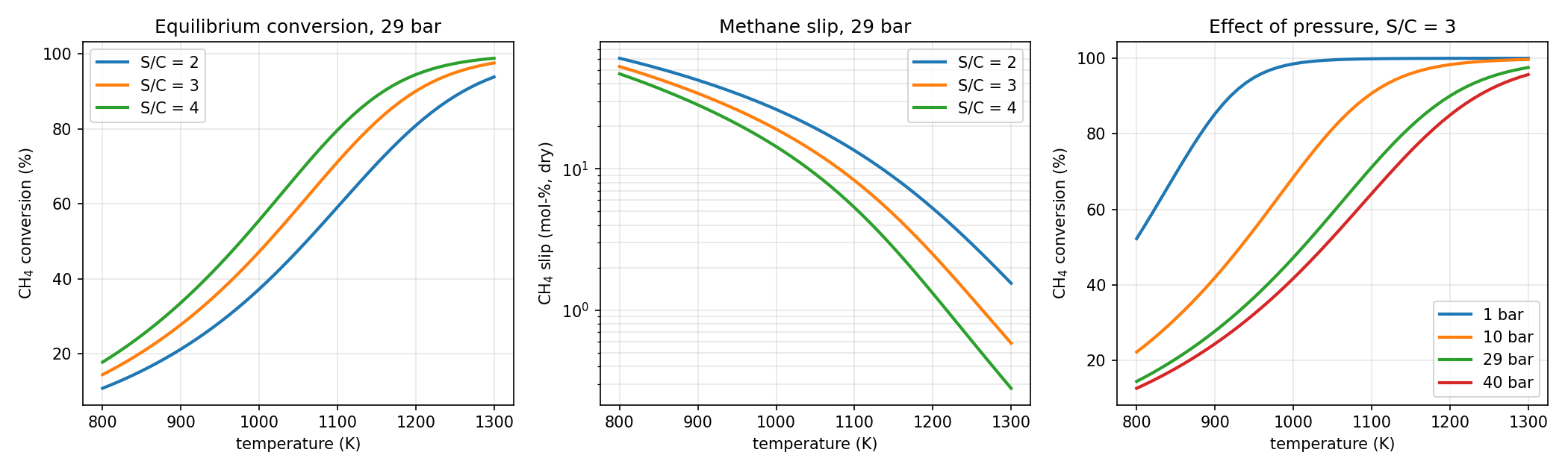
| 1 123 K (850 °C), 29 bar | S/C = 2 | S/C = 3 | S/C = 4 |
|---|---|---|---|
| CH₄ conversion | 64.5 % | 76.4 % | 84.2 % |
| CH₄ slip (dry gas) | 11.1 % | 6.5 % | 4.0 % |
| H₂/CO | 5.0 | 5.7 | 6.4 |
Pressure is the price of the process. At S/C = 3 and 1 123 K the equilibrium conversion is 99.9 % at 1 bar, 93.6 % at 10 bar and only 69.4 % at 40 bar. That is why ammonia plants follow the tubular reformer with a secondary, air-blown reformer. The primary reformer converts only about 65 % of the methane, leaving around 14 % CH₄ (dry); air burns part of the gas to about 1 200 °C, and the gas leaves the secondary catalyst at around 1 000 °C with 0.5 % CH₄ or less (Appl, 2000, Sec. 4.5.1.1). It is also why the H₂/CO ratio of a steam reformer, 5–6, is far above the value of about 2 needed for methanol or Fischer–Tropsch synthesis.
"""
Steam methane reforming — chemical equilibrium (the thermodynamic limit)
bdrworks.org · Handbook · Steam reforming, worked model 1

Equilibrium of CH4 + H2O = CO + 3H2 and CO + H2O = CO2 + H2 from a methane/steam feed
as a function of temperature, pressure and steam-to-carbon ratio (ideal gas).
Every reformer, whatever its design, is bounded by these curves.

Run:  python smr_equilibrium.py      (needs numpy, scipy, matplotlib)
"""
import numpy as np
import matplotlib.pyplot as plt

# ---------------------------------------------------------------- data
SPECIES = ["CH4", "H2O", "CO", "CO2", "H2", "N2", "O2"]
#                CH4  H2O   CO  CO2   H2  N2  O2
NU = np.array([[-1.0, -1.0, 1.0, 0.0, 3.0, 0.0, 0.0],    # 1: CH4 + H2O  <=> CO + 3 H2
               [0.0, -1.0, -1.0, 1.0, 1.0, 0.0, 0.0],    # 2: CO + H2O   <=> CO2 + H2
               [-1.0, -2.0, 0.0, 1.0, 4.0, 0.0, 0.0]])   # 3: CH4 + 2 H2O <=> CO2 + 4 H2
RG = 8.314                                                 # J/(mol K)
MW = np.array([16.043, 18.015, 28.010, 44.009, 2.016, 28.013, 31.999])   # kg/kmol

# NASA 7-coefficient polynomials (GRI-Mech 3.0 thermodynamic data): [low T < 1000 K], [high T]
NASA_LO = np.array([
    [5.14987613e+00, -1.36709788e-02, 4.91800599e-05, -4.84743026e-08, 1.66693956e-11, -1.02466476e+04, -4.64130376e+00],   # CH4
    [4.19864056e+00, -2.03643410e-03, 6.52040211e-06, -5.48797062e-09, 1.77197817e-12, -3.02937267e+04, -8.49032208e-01],   # H2O
    [3.57953347e+00, -6.10353680e-04, 1.01681433e-06, 9.07005884e-10, -9.04424499e-13, -1.43440860e+04, 3.50840928e+00],   # CO
    [2.35677352e+00, 8.98459677e-03, -7.12356269e-06, 2.45919022e-09, -1.43699548e-13, -4.83719697e+04, 9.90105222e+00],   # CO2
    [2.34433112e+00, 7.98052075e-03, -1.94781510e-05, 2.01572094e-08, -7.37611761e-12, -9.17935173e+02, 6.83010238e-01],   # H2
    [3.29867700e+00, 1.40824040e-03, -3.96322200e-06, 5.64151500e-09, -2.44485400e-12, -1.02089990e+03, 3.95037200e+00],   # N2
    [3.78245636e+00, -2.99673416e-03, 9.84730201e-06, -9.68129509e-09, 3.24372837e-12, -1.06394356e+03, 3.65767573e+00],   # O2
])
NASA_HI = np.array([
    [7.48514950e-02, 1.33909467e-02, -5.73285809e-06, 1.22292535e-09, -1.01815230e-13, -9.46834459e+03, 1.84373180e+01],   # CH4
    [3.03399249e+00, 2.17691804e-03, -1.64072518e-07, -9.70419870e-11, 1.68200992e-14, -3.00042971e+04, 4.96677010e+00],   # H2O
    [2.71518561e+00, 2.06252743e-03, -9.98825771e-07, 2.30053008e-10, -2.03647716e-14, -1.41518724e+04, 7.81868772e+00],   # CO
    [3.85746029e+00, 4.41437026e-03, -2.21481404e-06, 5.23490188e-10, -4.72084164e-14, -4.87591660e+04, 2.27163806e+00],   # CO2
    [3.33727920e+00, -4.94024731e-05, 4.99456778e-07, -1.79566394e-10, 2.00255376e-14, -9.50158922e+02, -3.20502331e+00],   # H2
    [2.92664000e+00, 1.48797680e-03, -5.68476000e-07, 1.00970380e-10, -6.75335100e-15, -9.22797700e+02, 5.98052800e+00],   # N2
    [3.28253784e+00, 1.48308754e-03, -7.57966669e-07, 2.09470555e-10, -2.16717794e-14, -1.08845772e+03, 5.45323129e+00],   # O2
])


def _a(T):
    return NASA_LO if T < 1000.0 else NASA_HI


def cp(T):
    """Ideal-gas heat capacities, J/(mol K)."""
    a = _a(T)
    return RG * (a[:, 0] + a[:, 1]*T + a[:, 2]*T**2 + a[:, 3]*T**3 + a[:, 4]*T**4)


def h(T):
    """Molar enthalpies including heats of formation, J/mol."""
    a = _a(T)
    return RG * T * (a[:, 0] + a[:, 1]*T/2 + a[:, 2]*T**2/3 + a[:, 3]*T**3/4 + a[:, 4]*T**4/5 + a[:, 5]/T)


def dH_rxn(T):
    """Heats of reactions 1-3, J/mol."""
    return NU @ h(T)


def K_eq(T):
    """Equilibrium constants of Xu & Froment: K1, K3 in bar^2, K2 dimensionless."""
    K1 = np.exp(-26830.0 / T + 30.114)
    K2 = np.exp(4400.0 / T - 4.036)
    return K1, K2, K1 * K2


def rates(T, p, eta=(1.0, 1.0, 1.0)):
    """Xu & Froment (1989) intrinsic rates times effectiveness factors, kmol/(kg_cat h); p in bar."""
    pCH4, pH2O, pCO, pCO2, pH2 = [max(x, 1e-10) for x in p[:5]]
    RT = RG * T / 1000.0                                         # kJ/mol
    k1 = 4.225e15 * np.exp(-240.1 / RT)
    k2 = 1.955e6 * np.exp(-67.13 / RT)
    k3 = 1.020e15 * np.exp(-243.9 / RT)
    KCO = 8.23e-5 * np.exp(70.65 / RT)
    KH2 = 6.12e-9 * np.exp(82.90 / RT)
    KCH4 = 6.65e-4 * np.exp(38.28 / RT)
    KH2O = 1.77e5 * np.exp(-88.68 / RT)
    K1, K2, K3 = K_eq(T)
    den = 1.0 + KCO*pCO + KH2*pH2 + KCH4*pCH4 + KH2O*pH2O/pH2
    r1 = k1 / pH2**2.5 * (pCH4*pH2O - pH2**3*pCO/K1) / den**2
    r2 = k2 / pH2 * (pCO*pH2O - pH2*pCO2/K2) / den**2
    r3 = k3 / pH2**3.5 * (pCH4*pH2O**2 - pH2**4*pCO2/K3) / den**2
    return np.array([eta[0]*r1, eta[1]*r2, eta[2]*r3])


def equilibrium(T, P, n0):
    """Equilibrium of reactions 1 and 2 (3 is their sum) from flows n0 at T (K), P (bar)."""
    from scipy.optimize import fsolve
    K1, K2, _ = K_eq(T)
    def res(x):
        n = np.maximum(n0 + NU[0]*x[0] + NU[1]*x[1], 1e-14)
        p = P * n / n.sum()
        return [np.log(p[2]*p[4]**3 / (p[0]*p[1])) - np.log(K1), np.log(p[3]*p[4] / (p[2]*p[1])) - np.log(K2)]
    x = fsolve(res, [0.7*n0[0], 0.2*n0[0]], xtol=1e-12)
    return n0 + NU[0]*x[0] + NU[1]*x[1]


def feed(sc):
    return np.array([1.0, sc, 0.0, 0.0, 0.05, 0.0, 0.0])


def summary(n, n0):
    dry = n.sum() - n[1]
    return 1 - n[0] / n0[0], 100 * n[0] / dry, n[4] / n[2], n[4] / n0[0]


if __name__ == "__main__":
    Ts = np.linspace(800, 1300, 51)
    fig, ax = plt.subplots(1, 3, figsize=(14, 4.2))
    for sc in [2.0, 3.0, 4.0]:
        n0 = feed(sc)
        res = [summary(equilibrium(t, 29.0, n0), n0) for t in Ts]
        ax[0].plot(Ts, [100 * r[0] for r in res], lw=2, label=f"S/C = {sc:.0f}")
        ax[1].plot(Ts, [r[1] for r in res], lw=2, label=f"S/C = {sc:.0f}")
    for P in [1.0, 10.0, 29.0, 40.0]:
        n0 = feed(3.0)
        ax[2].plot(Ts, [100 * summary(equilibrium(t, P, n0), n0)[0] for t in Ts], lw=2, label=f"{P:.0f} bar")
    ax[0].set(xlabel="temperature (K)", ylabel="CH$_4$ conversion (%)", title="Equilibrium conversion, 29 bar")
    ax[1].set(xlabel="temperature (K)", ylabel="CH$_4$ slip (mol-%, dry)", title="Methane slip, 29 bar", yscale="log")
    ax[2].set(xlabel="temperature (K)", ylabel="CH$_4$ conversion (%)", title="Effect of pressure, S/C = 3")
    for a in ax:
        a.grid(alpha=0.3, which="both"); a.legend()
    fig.tight_layout(); fig.savefig("smr_equilibrium.png", dpi=150)
    for sc in [2.0, 3.0, 4.0]:
        n0 = feed(sc); X, slip, h2co, h2 = summary(equilibrium(1123.0, 29.0, n0), n0)
        print(f"1123 K, 29 bar, S/C {sc:.0f}: CH4 conversion {100*X:.1f} %, slip {slip:.2f} % dry, H2/CO {h2co:.2f}, H2 per CH4 {h2:.2f}")
    for P in [1.0, 10.0, 40.0]:
        n0 = feed(3.0); print(f"1123 K, {P:.0f} bar, S/C 3: CH4 conversion {100*summary(equilibrium(1123.0, P, n0), n0)[0]:.1f} %")
    plt.show()
function smr_equilibrium()
% Steam methane reforming - chemical equilibrium (the thermodynamic limit)
% bdrworks.org - Handbook - Steam reforming, worked model 1
% Save as smr_equilibrium.m and run:  smr_equilibrium

Ts = linspace(800, 1300, 51);
figure('Position', [100 100 1000 380]); hold on;
for sc = [2 3 4]
    n0 = [1; sc; 0; 0; 0.05; 0; 0];  X = zeros(size(Ts));
    for k = 1:numel(Ts), n = equilibrium(Ts(k), 29, n0); X(k) = 1 - n(1)/n0(1); end
    plot(Ts, 100*X, 'LineWidth', 2);
    n = equilibrium(1123, 29, n0);  dry = sum(n) - n(2);
    fprintf('1123 K, 29 bar, S/C %d: CH4 conversion %.1f %%, slip %.2f %% dry, H2/CO %.2f\n', sc, 100*(1 - n(1)), 100*n(1)/dry, n(5)/n(3));
end
xlabel('T (K)'); ylabel('CH_4 conversion (%)'); legend('S/C = 2', 'S/C = 3', 'S/C = 4'); grid on;
end

% ================================================================ properties & kinetics
function nu = stoich()
%       CH4 H2O  CO CO2  H2 N2  O2
nu = [  -1  -1    1   0   3  0   0;      % CH4 + H2O   <=> CO + 3H2
         0  -1   -1   1   1  0   0;      % CO + H2O    <=> CO2 + H2
        -1  -2    0   1   4  0   0];     % CH4 + 2H2O  <=> CO2 + 4H2
end

function a = nasa(T)
% NASA 7-coefficient polynomials (GRI-Mech 3.0) for CH4 H2O CO CO2 H2 N2 O2
if T < 1000
  a = [
     5.14987613e+00, -1.36709788e-02, 4.91800599e-05, -4.84743026e-08, 1.66693956e-11, -1.02466476e+04, -4.64130376e+00;   % CH4
     4.19864056e+00, -2.03643410e-03, 6.52040211e-06, -5.48797062e-09, 1.77197817e-12, -3.02937267e+04, -8.49032208e-01;   % H2O
     3.57953347e+00, -6.10353680e-04, 1.01681433e-06, 9.07005884e-10, -9.04424499e-13, -1.43440860e+04, 3.50840928e+00;   % CO
     2.35677352e+00, 8.98459677e-03, -7.12356269e-06, 2.45919022e-09, -1.43699548e-13, -4.83719697e+04, 9.90105222e+00;   % CO2
     2.34433112e+00, 7.98052075e-03, -1.94781510e-05, 2.01572094e-08, -7.37611761e-12, -9.17935173e+02, 6.83010238e-01;   % H2
     3.29867700e+00, 1.40824040e-03, -3.96322200e-06, 5.64151500e-09, -2.44485400e-12, -1.02089990e+03, 3.95037200e+00;   % N2
     3.78245636e+00, -2.99673416e-03, 9.84730201e-06, -9.68129509e-09, 3.24372837e-12, -1.06394356e+03, 3.65767573e+00;   % O2
  ];
else
  a = [
     7.48514950e-02, 1.33909467e-02, -5.73285809e-06, 1.22292535e-09, -1.01815230e-13, -9.46834459e+03, 1.84373180e+01;   % CH4
     3.03399249e+00, 2.17691804e-03, -1.64072518e-07, -9.70419870e-11, 1.68200992e-14, -3.00042971e+04, 4.96677010e+00;   % H2O
     2.71518561e+00, 2.06252743e-03, -9.98825771e-07, 2.30053008e-10, -2.03647716e-14, -1.41518724e+04, 7.81868772e+00;   % CO
     3.85746029e+00, 4.41437026e-03, -2.21481404e-06, 5.23490188e-10, -4.72084164e-14, -4.87591660e+04, 2.27163806e+00;   % CO2
     3.33727920e+00, -4.94024731e-05, 4.99456778e-07, -1.79566394e-10, 2.00255376e-14, -9.50158922e+02, -3.20502331e+00;   % H2
     2.92664000e+00, 1.48797680e-03, -5.68476000e-07, 1.00970380e-10, -6.75335100e-15, -9.22797700e+02, 5.98052800e+00;   % N2
     3.28253784e+00, 1.48308754e-03, -7.57966669e-07, 2.09470555e-10, -2.16717794e-14, -1.08845772e+03, 5.45323129e+00;   % O2
  ];
end
end

function c = cp_all(T)
a = nasa(T);  c = 8.314*(a(:,1) + a(:,2)*T + a(:,3)*T^2 + a(:,4)*T^3 + a(:,5)*T^4);     % J/(mol K)
end

function H = h_all(T)
a = nasa(T);  H = 8.314*T*(a(:,1) + a(:,2)*T/2 + a(:,3)*T^2/3 + a(:,4)*T^3/4 + a(:,5)*T^4/5 + a(:,6)/T);   % J/mol
end

function dH = dH_rxn(T)
dH = stoich()*h_all(T);
end

function [K1, K2, K3] = K_eq(T)
K1 = exp(-26830/T + 30.114);  K2 = exp(4400/T - 4.036);  K3 = K1*K2;      % Xu & Froment
end

function r = rates(T, p, eta)
% Xu & Froment (1989) rates times effectiveness factors, kmol/(kg_cat h); p in bar [CH4 H2O CO CO2 H2 ...]
p = max(p, 1e-10);  RT = 8.314e-3*T;
k1 = 4.225e15*exp(-240.1/RT);  k2 = 1.955e6*exp(-67.13/RT);  k3 = 1.020e15*exp(-243.9/RT);
KCO = 8.23e-5*exp(70.65/RT);  KH2 = 6.12e-9*exp(82.90/RT);  KCH4 = 6.65e-4*exp(38.28/RT);  KH2O = 1.77e5*exp(-88.68/RT);
[K1, K2, K3] = K_eq(T);
den = 1 + KCO*p(3) + KH2*p(5) + KCH4*p(1) + KH2O*p(2)/p(5);
r = eta(:).*[k1/p(5)^2.5*(p(1)*p(2) - p(5)^3*p(3)/K1)/den^2;
             k2/p(5)*(p(3)*p(2) - p(5)*p(4)/K2)/den^2;
             k3/p(5)^3.5*(p(1)*p(2)^2 - p(5)^4*p(4)/K3)/den^2];
end

function n = equilibrium(T, P, n0)
% equilibrium of reactions 1 and 2 by Newton's method on the log equations
nu = stoich();  [K1, K2] = K_eq(T);  x = [0.7*n0(1); 0.2*n0(1)];
f = @(x) eqres(x, n0, nu, P, K1, K2);
for it = 1:100
    F = f(x);  J = zeros(2);  h = 1e-7*max(abs(x), 1e-6);
    for j = 1:2, e = zeros(2,1); e(j) = h(j); J(:,j) = (f(x + e) - F)/h(j); end
    dx = -J\F;  lam = 1;
    while any(n0 + nu(1,:)'*(x(1)+lam*dx(1)) + nu(2,:)'*(x(2)+lam*dx(2)) < 0 & [1 1 1 1 1 0 0]') && lam > 1e-4, lam = lam/2; end
    x = x + lam*dx;
    if norm(dx) < 1e-12*max(1, norm(x)), break; end
end
n = n0 + nu(1,:)'*x(1) + nu(2,:)'*x(2);
end

function F = eqres(x, n0, nu, P, K1, K2)
n = max(n0 + nu(1,:)'*x(1) + nu(2,:)'*x(2), 1e-14);  p = P*n/sum(n);
F = [log(p(3)*p(5)^3/(p(1)*p(2))) - log(K1);  log(p(4)*p(5)/(p(3)*p(2))) - log(K2)];
end
5Solution 2 · Fired reformer tube
One tube is modelled as a one-dimensional plug-flow reactor: inside diameter 101.6 mm, outside diameter 132 mm, 12 m heated length, 1 360 kg/m³ of catalyst with 17.3 mm equivalent pellets. The furnace is represented by a prescribed heat flux on the outer tube surface. It is highest at the top, where the burners are, and falls linearly to 70 % of the average at the bottom. The balances include the Ergun pressure drop (Ergun, 1952):
The tube wall, not the catalyst, limits a reformer. The heat flux has to cross the gas film inside the tube and the wall metal, so the metal runs much hotter than the gas:
With a mass flux of 14 kg/(m²s) the Leva correlation gives hi ≈ 1 180 W/m²K (Leva, 1947; Froment et al., 2011, Ch. 11). A wall conductivity of 25 W/(m K) is typical of HP-type cast alloys at these temperatures. HP alloys (32–35 % Ni, 23–27 % Cr, about 1.5 % Nb) have largely replaced the older HK 40 and allow about 40 bar at outer wall temperatures around 900 °C (Appl, 2000, Sec. 4.5.1.1).
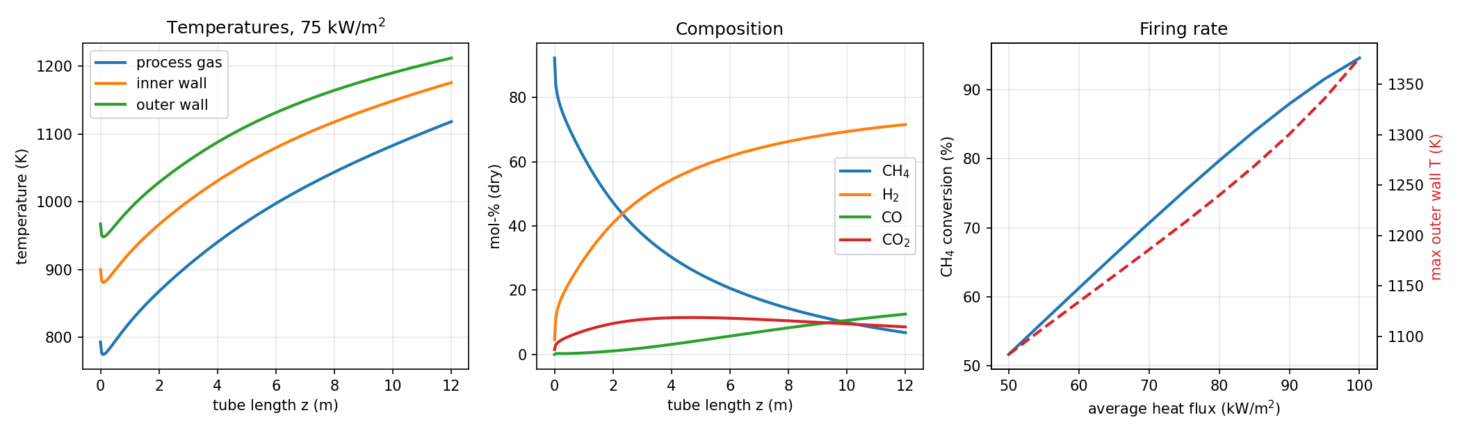
| Result, q̄ = 75 kW/m² | Value |
|---|---|
| Outlet temperature and pressure | 1 118 K (845 °C), 26.9 bar |
| CH₄ conversion | 75.3 % (equilibrium at the outlet: 77.0 %) |
| CH₄ slip (dry) | 6.8 % |
| H₂/CO | 5.7 |
| Maximum outer wall temperature | 1 212 K (939 °C), at the outlet |
The profiles tell the story of a reformer tube:
- The gas temperature first dips at the inlet, by about 20 K within the first 0.1–0.2 m. The feed enters as unreformed methane and steam, far from equilibrium, so the strongly endothermic reforming runs fastest there and absorbs heat faster than the wall supplies it; the walls follow the gas because the flux is fixed. As soon as the gas nears equilibrium the rate falls to what the heat input allows and the temperature rises. The sharp corner is this fast initial zone seen on a 12 m scale; with a pre-reformed feed, or a lower catalyst activity at the top, the dip becomes shallower.
- After the dip, the gas heats steadily towards 1 120 K. The composition tracks the equilibrium curve closely, and the outlet is within two percentage points of equilibrium. Every kilowatt through the wall is used at once to convert methane.
- The outer wall runs about 95–175 K hotter than the gas, most at the inlet where the flux is highest, and its maximum is set by the combination of heat flux and gas temperature. The sweep in Figure 2 shows the trade-off. Raising the average flux from 75 to 100 kW/m² lifts conversion from 75 to 95 %, but the wall rises from 1 212 to 1 376 K, far beyond what tube alloys survive. Creep life falls steeply with metal temperature (Appl, 2000, Sec. 4.5.1.1); a common rule of thumb is that 20 K above design roughly halves it. The tube metal, not the chemistry, fixes the capacity of a reformer.
- The Ergun pressure drop is 2.1 bar. It is included here because it affects both the equilibrium and the design of the upstream compressor.
"""
Steam methane reforming — one fired reformer tube
bdrworks.org · Handbook · Steam reforming, worked model 2

Catalyst tube in a top-fired furnace. Heat enters through the tube wall with a
prescribed flux profile; the gas is heated and reformed on Ni/Al2O3 catalyst.
    dF_i/dz = rho_b A sum_j nu_ij eta_j r_j                        (Xu & Froment, 1989)
    (sum F_i cp_i) dT/dz = pi d_o q(z) + rho_b A sum_j (-dH_j) eta_j r_j
    dP/dz  = -(Ergun)
Tube-wall temperatures follow from the inside film coefficient (Leva) and wall conduction.

Run:  python smr_tube.py      (needs numpy, scipy, matplotlib)
"""
import numpy as np
from scipy.integrate import solve_ivp
import matplotlib.pyplot as plt

# ---------------------------------------------------------------- data
SPECIES = ["CH4", "H2O", "CO", "CO2", "H2", "N2", "O2"]
#                CH4  H2O   CO  CO2   H2  N2  O2
NU = np.array([[-1.0, -1.0, 1.0, 0.0, 3.0, 0.0, 0.0],    # 1: CH4 + H2O  <=> CO + 3 H2
               [0.0, -1.0, -1.0, 1.0, 1.0, 0.0, 0.0],    # 2: CO + H2O   <=> CO2 + H2
               [-1.0, -2.0, 0.0, 1.0, 4.0, 0.0, 0.0]])   # 3: CH4 + 2 H2O <=> CO2 + 4 H2
RG = 8.314                                                 # J/(mol K)
MW = np.array([16.043, 18.015, 28.010, 44.009, 2.016, 28.013, 31.999])   # kg/kmol

# NASA 7-coefficient polynomials (GRI-Mech 3.0 thermodynamic data): [low T < 1000 K], [high T]
NASA_LO = np.array([
    [5.14987613e+00, -1.36709788e-02, 4.91800599e-05, -4.84743026e-08, 1.66693956e-11, -1.02466476e+04, -4.64130376e+00],   # CH4
    [4.19864056e+00, -2.03643410e-03, 6.52040211e-06, -5.48797062e-09, 1.77197817e-12, -3.02937267e+04, -8.49032208e-01],   # H2O
    [3.57953347e+00, -6.10353680e-04, 1.01681433e-06, 9.07005884e-10, -9.04424499e-13, -1.43440860e+04, 3.50840928e+00],   # CO
    [2.35677352e+00, 8.98459677e-03, -7.12356269e-06, 2.45919022e-09, -1.43699548e-13, -4.83719697e+04, 9.90105222e+00],   # CO2
    [2.34433112e+00, 7.98052075e-03, -1.94781510e-05, 2.01572094e-08, -7.37611761e-12, -9.17935173e+02, 6.83010238e-01],   # H2
    [3.29867700e+00, 1.40824040e-03, -3.96322200e-06, 5.64151500e-09, -2.44485400e-12, -1.02089990e+03, 3.95037200e+00],   # N2
    [3.78245636e+00, -2.99673416e-03, 9.84730201e-06, -9.68129509e-09, 3.24372837e-12, -1.06394356e+03, 3.65767573e+00],   # O2
])
NASA_HI = np.array([
    [7.48514950e-02, 1.33909467e-02, -5.73285809e-06, 1.22292535e-09, -1.01815230e-13, -9.46834459e+03, 1.84373180e+01],   # CH4
    [3.03399249e+00, 2.17691804e-03, -1.64072518e-07, -9.70419870e-11, 1.68200992e-14, -3.00042971e+04, 4.96677010e+00],   # H2O
    [2.71518561e+00, 2.06252743e-03, -9.98825771e-07, 2.30053008e-10, -2.03647716e-14, -1.41518724e+04, 7.81868772e+00],   # CO
    [3.85746029e+00, 4.41437026e-03, -2.21481404e-06, 5.23490188e-10, -4.72084164e-14, -4.87591660e+04, 2.27163806e+00],   # CO2
    [3.33727920e+00, -4.94024731e-05, 4.99456778e-07, -1.79566394e-10, 2.00255376e-14, -9.50158922e+02, -3.20502331e+00],   # H2
    [2.92664000e+00, 1.48797680e-03, -5.68476000e-07, 1.00970380e-10, -6.75335100e-15, -9.22797700e+02, 5.98052800e+00],   # N2
    [3.28253784e+00, 1.48308754e-03, -7.57966669e-07, 2.09470555e-10, -2.16717794e-14, -1.08845772e+03, 5.45323129e+00],   # O2
])


def _a(T):
    return NASA_LO if T < 1000.0 else NASA_HI


def cp(T):
    """Ideal-gas heat capacities, J/(mol K)."""
    a = _a(T)
    return RG * (a[:, 0] + a[:, 1]*T + a[:, 2]*T**2 + a[:, 3]*T**3 + a[:, 4]*T**4)


def h(T):
    """Molar enthalpies including heats of formation, J/mol."""
    a = _a(T)
    return RG * T * (a[:, 0] + a[:, 1]*T/2 + a[:, 2]*T**2/3 + a[:, 3]*T**3/4 + a[:, 4]*T**4/5 + a[:, 5]/T)


def dH_rxn(T):
    """Heats of reactions 1-3, J/mol."""
    return NU @ h(T)


def K_eq(T):
    """Equilibrium constants of Xu & Froment: K1, K3 in bar^2, K2 dimensionless."""
    K1 = np.exp(-26830.0 / T + 30.114)
    K2 = np.exp(4400.0 / T - 4.036)
    return K1, K2, K1 * K2


def rates(T, p, eta=(1.0, 1.0, 1.0)):
    """Xu & Froment (1989) intrinsic rates times effectiveness factors, kmol/(kg_cat h); p in bar."""
    pCH4, pH2O, pCO, pCO2, pH2 = [max(x, 1e-10) for x in p[:5]]
    RT = RG * T / 1000.0                                         # kJ/mol
    k1 = 4.225e15 * np.exp(-240.1 / RT)
    k2 = 1.955e6 * np.exp(-67.13 / RT)
    k3 = 1.020e15 * np.exp(-243.9 / RT)
    KCO = 8.23e-5 * np.exp(70.65 / RT)
    KH2 = 6.12e-9 * np.exp(82.90 / RT)
    KCH4 = 6.65e-4 * np.exp(38.28 / RT)
    KH2O = 1.77e5 * np.exp(-88.68 / RT)
    K1, K2, K3 = K_eq(T)
    den = 1.0 + KCO*pCO + KH2*pH2 + KCH4*pCH4 + KH2O*pH2O/pH2
    r1 = k1 / pH2**2.5 * (pCH4*pH2O - pH2**3*pCO/K1) / den**2
    r2 = k2 / pH2 * (pCO*pH2O - pH2*pCO2/K2) / den**2
    r3 = k3 / pH2**3.5 * (pCH4*pH2O**2 - pH2**4*pCO2/K3) / den**2
    return np.array([eta[0]*r1, eta[1]*r2, eta[2]*r3])


def equilibrium(T, P, n0):
    """Equilibrium of reactions 1 and 2 (3 is their sum) from flows n0 at T (K), P (bar)."""
    from scipy.optimize import fsolve
    K1, K2, _ = K_eq(T)
    def res(x):
        n = np.maximum(n0 + NU[0]*x[0] + NU[1]*x[1], 1e-14)
        p = P * n / n.sum()
        return [np.log(p[2]*p[4]**3 / (p[0]*p[1])) - np.log(K1), np.log(p[3]*p[4] / (p[2]*p[1])) - np.log(K2)]
    x = fsolve(res, [0.7*n0[0], 0.2*n0[0]], xtol=1e-12)
    return n0 + NU[0]*x[0] + NU[1]*x[1]

# ---------------------------------------------------------------- tube
L, D_I, D_O = 12.0, 0.1016, 0.1320     # heated length, inside and outside diameter, m
A = np.pi * D_I**2 / 4                 # flow area, m2
RHO_B = 1360.0                         # catalyst bulk density, kg/m3
D_P, EPS = 0.0173, 0.50                # equivalent pellet diameter (m), bed voidage
ETA = (0.03, 0.03, 0.03)               # effectiveness factors of reactions 1-3
MU, LAM_G, K_W = 3.0e-5, 0.12, 25.0    # gas viscosity (Pa s), gas conductivity and wall conductivity (W/m K)
P0, T0 = 29.0, 793.0                   # inlet pressure (bar) and temperature (K)
F_CH4, S_C = 6.0, 3.0                  # methane per tube (kmol/h), steam-to-carbon ratio
F0 = np.array([F_CH4, S_C * F_CH4, 0.0, 0.1, 0.3, 0.1, 0.0]) / 3.6   # mol/s per tube (H2 keeps Ni reduced)


def q_flux(z, q_avg):
    """Heat flux on the outer tube surface, W/m2: highest near the burners at the top."""
    return q_avg * (1.3 - 0.6 * z / L)


def rhs(z, u, q_avg):
    F, T, P = u[:7], u[7], u[8]
    y = F / F.sum()
    r = rates(T, P * y, ETA) / 3.6                                # mol/(kg s)
    dF = RHO_B * A * (NU.T @ r)
    Q = np.pi * D_O * q_flux(z, q_avg)                            # W per m of tube
    dT = (Q + RHO_B * A * np.dot(-dH_rxn(T), r)) / np.dot(F, cp(T))
    G = np.dot(F, MW) / 1000 / A                                  # kg/(m2 s)
    rho = P * 1e5 * np.dot(y, MW) / 1000 / (RG * T)
    us = G / rho
    dP = -(150 * MU * (1 - EPS)**2 / (EPS**3 * D_P**2) * us + 1.75 * rho * (1 - EPS) / (EPS**3 * D_P) * us**2) / 1e5
    return np.concatenate([dF, [dT, dP]])


def wall_T(z, T, q_avg):
    """Inner and outer tube-wall temperatures, K (Leva correlation for heating packed tubes)."""
    G = np.dot(F0, MW) / 1000 / A
    h_i = 0.813 * LAM_G / D_I * (D_P * G / MU)**0.9 * np.exp(-6 * D_P / D_I)
    q = q_flux(z, q_avg)
    Twi = T + q * D_O / (h_i * D_I)
    Two = Twi + q * D_O / 2 * np.log(D_O / D_I) / K_W
    return Twi, Two, h_i


def solve(q_avg, n=300):
    sol = solve_ivp(rhs, (0, L), np.concatenate([F0, [T0, P0]]), args=(q_avg,), method="LSODA",
                    rtol=1e-8, atol=1e-10, dense_output=True)
    z = np.linspace(0, L, n)
    return z, sol.sol(z)


def outlet(u):
    F = u[:7, -1]
    X = 1 - F[0] / F0[0]
    dry = F.sum() - F[1]
    return X, 100 * F[0] / dry, u[7, -1], u[8, -1], F[4] / F[2]


if __name__ == "__main__":
    q = 75e3                                                      # average heat flux, W/m2
    z, u = solve(q)
    Twi, Two, h_i = wall_T(z, u[7], q)
    X, slip, Tout, Pout, h2co = outlet(u)
    ne = equilibrium(Tout, Pout, F0)
    Xeq = 1 - ne[0] / F0[0]
    print(f"tube {L} m x {1000*D_I:.1f} mm, S/C {S_C}, {F_CH4} kmol/h CH4, average flux {q/1e3:.0f} kW/m2, h_i = {h_i:.0f} W/m2K")
    print(f"outlet {Tout:.1f} K, {Pout:.2f} bar, CH4 conversion {100*X:.1f} % (equilibrium at outlet {100*Xeq:.1f} %), "
          f"CH4 slip {slip:.2f} % dry, H2/CO {h2co:.2f}")
    print(f"max outer wall temperature {Two.max():.0f} K at z = {z[Two.argmax()]:.1f} m")

    fig, ax = plt.subplots(1, 3, figsize=(14, 4.2))
    ax[0].plot(z, u[7], lw=2, label="process gas")
    ax[0].plot(z, Twi, lw=2, label="inner wall")
    ax[0].plot(z, Two, lw=2, label="outer wall")
    ax[0].set(xlabel="tube length z (m)", ylabel="temperature (K)", title="Temperatures, 75 kW/m$^2$"); ax[0].legend()
    Fz = u[:7]
    dry = Fz.sum(axis=0) - Fz[1]
    for i, s in [(0, "CH$_4$"), (4, "H$_2$"), (2, "CO"), (3, "CO$_2$")]:
        ax[1].plot(z, 100 * Fz[i] / dry, lw=2, label=s)
    ax[1].set(xlabel="tube length z (m)", ylabel="mol-% (dry)", title="Composition"); ax[1].legend()
    qs = np.arange(50e3, 101e3, 5e3)
    res = []
    for qq in qs:
        zz, uu = solve(qq)
        res.append(outlet(uu) + (wall_T(zz, uu[7], qq)[1].max(),))
    ax[2].plot(qs / 1e3, [100 * r[0] for r in res], lw=2, c="C0", label="CH$_4$ conversion")
    ax[2].set(xlabel="average heat flux (kW/m$^2$)", ylabel="CH$_4$ conversion (%)", title="Firing rate")
    a2 = ax[2].twinx(); a2.plot(qs / 1e3, [r[5] for r in res], lw=2, c="C3", ls="--"); a2.set_ylabel("max outer wall T (K)", color="C3")
    for a in ax:
        a.grid(alpha=0.3)
    fig.tight_layout()
    fig.savefig("smr_tube.png", dpi=150)
    print("flux sweep (kW/m2: conversion %, outlet K, max wall K):",
          ", ".join(f"{qq/1e3:.0f}: {100*r[0]:.1f}/{r[2]:.0f}/{r[5]:.0f}" for qq, r in zip(qs, res)))
    plt.show()
function smr_tube()
% Steam methane reforming - one fired reformer tube (Xu & Froment kinetics, Ergun pressure drop)
% bdrworks.org - Handbook - Steam reforming, worked model 2
% Save as smr_tube.m and run:  smr_tube

p = params();  q = 75e3;                                   % average heat flux, W/m2
[z, u] = tube(p, q);
[Twi, Two, hi] = wall_T(p, z, u(:,8), q);
F = u(end,1:7)';  X = 1 - F(1)/p.F0(1);  dry = sum(F) - F(2);
fprintf('h_i = %.0f W/m2K; outlet %.1f K, %.2f bar, CH4 conversion %.1f %%, slip %.2f %% dry, H2/CO %.2f\n', ...
    hi, u(end,8), u(end,9), 100*X, 100*F(1)/dry, F(5)/F(3));
fprintf('max outer wall temperature %.0f K\n', max(Two));
figure; plot(z, u(:,8), z, Twi, z, Two, 'LineWidth', 2); legend('gas', 'inner wall', 'outer wall'); xlabel('z (m)'); ylabel('T (K)'); grid on;
end

function p = params()
p.L = 12; p.Di = 0.1016; p.Do = 0.1320; p.A = pi*p.Di^2/4; p.rho = 1360; p.dp = 0.0173; p.eps = 0.5;
p.eta = [0.03 0.03 0.03]; p.mu = 3e-5; p.lam = 0.12; p.kw = 25; p.P0 = 29; p.T0 = 793;
p.MW = [16.043 18.015 28.010 44.009 2.016 28.013 31.999]';
p.F0 = [6; 18; 0; 0.1; 0.3; 0.1; 0]/3.6;                   % mol/s per tube, S/C = 3
end

function q = qflux(p, z, qavg)
q = qavg*(1.3 - 0.6*z/p.L);
end

function [z, u] = tube(p, qavg)
opts = odeset('RelTol', 1e-8, 'AbsTol', 1e-10);
[z, u] = ode45(@(z,u) rhs(z, u, p, qavg), linspace(0, p.L, 300), [p.F0; p.T0; p.P0], opts);
end

function du = rhs(z, u, p, qavg)
F = u(1:7); T = u(8); P = u(9); y = F/sum(F); nu = stoich();
r = rates(T, P*y, p.eta)/3.6;                              % mol/(kg s)
Q = pi*p.Do*qflux(p, z, qavg);
G = (F'*p.MW)/1000/p.A;  rho = P*1e5*(y'*p.MW)/1000/(8.314*T);  us = G/rho;
dP = -(150*p.mu*(1-p.eps)^2/(p.eps^3*p.dp^2)*us + 1.75*rho*(1-p.eps)/(p.eps^3*p.dp)*us^2)/1e5;
du = [p.rho*p.A*(nu'*r); (Q + p.rho*p.A*(-dH_rxn(T))'*r)/(F'*cp_all(T)); dP];
end

function [Twi, Two, hi] = wall_T(p, z, T, qavg)
G = (p.F0'*p.MW)/1000/p.A;
hi = 0.813*p.lam/p.Di*(p.dp*G/p.mu)^0.9*exp(-6*p.dp/p.Di);   % Leva
q = qflux(p, z, qavg);
Twi = T + q*p.Do/(hi*p.Di);  Two = Twi + q*p.Do/2*log(p.Do/p.Di)/p.kw;
end

% ================================================================ properties & kinetics
function nu = stoich()
%       CH4 H2O  CO CO2  H2 N2  O2
nu = [  -1  -1    1   0   3  0   0;      % CH4 + H2O   <=> CO + 3H2
         0  -1   -1   1   1  0   0;      % CO + H2O    <=> CO2 + H2
        -1  -2    0   1   4  0   0];     % CH4 + 2H2O  <=> CO2 + 4H2
end

function a = nasa(T)
% NASA 7-coefficient polynomials (GRI-Mech 3.0) for CH4 H2O CO CO2 H2 N2 O2
if T < 1000
  a = [
     5.14987613e+00, -1.36709788e-02, 4.91800599e-05, -4.84743026e-08, 1.66693956e-11, -1.02466476e+04, -4.64130376e+00;   % CH4
     4.19864056e+00, -2.03643410e-03, 6.52040211e-06, -5.48797062e-09, 1.77197817e-12, -3.02937267e+04, -8.49032208e-01;   % H2O
     3.57953347e+00, -6.10353680e-04, 1.01681433e-06, 9.07005884e-10, -9.04424499e-13, -1.43440860e+04, 3.50840928e+00;   % CO
     2.35677352e+00, 8.98459677e-03, -7.12356269e-06, 2.45919022e-09, -1.43699548e-13, -4.83719697e+04, 9.90105222e+00;   % CO2
     2.34433112e+00, 7.98052075e-03, -1.94781510e-05, 2.01572094e-08, -7.37611761e-12, -9.17935173e+02, 6.83010238e-01;   % H2
     3.29867700e+00, 1.40824040e-03, -3.96322200e-06, 5.64151500e-09, -2.44485400e-12, -1.02089990e+03, 3.95037200e+00;   % N2
     3.78245636e+00, -2.99673416e-03, 9.84730201e-06, -9.68129509e-09, 3.24372837e-12, -1.06394356e+03, 3.65767573e+00;   % O2
  ];
else
  a = [
     7.48514950e-02, 1.33909467e-02, -5.73285809e-06, 1.22292535e-09, -1.01815230e-13, -9.46834459e+03, 1.84373180e+01;   % CH4
     3.03399249e+00, 2.17691804e-03, -1.64072518e-07, -9.70419870e-11, 1.68200992e-14, -3.00042971e+04, 4.96677010e+00;   % H2O
     2.71518561e+00, 2.06252743e-03, -9.98825771e-07, 2.30053008e-10, -2.03647716e-14, -1.41518724e+04, 7.81868772e+00;   % CO
     3.85746029e+00, 4.41437026e-03, -2.21481404e-06, 5.23490188e-10, -4.72084164e-14, -4.87591660e+04, 2.27163806e+00;   % CO2
     3.33727920e+00, -4.94024731e-05, 4.99456778e-07, -1.79566394e-10, 2.00255376e-14, -9.50158922e+02, -3.20502331e+00;   % H2
     2.92664000e+00, 1.48797680e-03, -5.68476000e-07, 1.00970380e-10, -6.75335100e-15, -9.22797700e+02, 5.98052800e+00;   % N2
     3.28253784e+00, 1.48308754e-03, -7.57966669e-07, 2.09470555e-10, -2.16717794e-14, -1.08845772e+03, 5.45323129e+00;   % O2
  ];
end
end

function c = cp_all(T)
a = nasa(T);  c = 8.314*(a(:,1) + a(:,2)*T + a(:,3)*T^2 + a(:,4)*T^3 + a(:,5)*T^4);     % J/(mol K)
end

function H = h_all(T)
a = nasa(T);  H = 8.314*T*(a(:,1) + a(:,2)*T/2 + a(:,3)*T^2/3 + a(:,4)*T^3/4 + a(:,5)*T^4/5 + a(:,6)/T);   % J/mol
end

function dH = dH_rxn(T)
dH = stoich()*h_all(T);
end

function [K1, K2, K3] = K_eq(T)
K1 = exp(-26830/T + 30.114);  K2 = exp(4400/T - 4.036);  K3 = K1*K2;      % Xu & Froment
end

function r = rates(T, p, eta)
% Xu & Froment (1989) rates times effectiveness factors, kmol/(kg_cat h); p in bar [CH4 H2O CO CO2 H2 ...]
p = max(p, 1e-10);  RT = 8.314e-3*T;
k1 = 4.225e15*exp(-240.1/RT);  k2 = 1.955e6*exp(-67.13/RT);  k3 = 1.020e15*exp(-243.9/RT);
KCO = 8.23e-5*exp(70.65/RT);  KH2 = 6.12e-9*exp(82.90/RT);  KCH4 = 6.65e-4*exp(38.28/RT);  KH2O = 1.77e5*exp(-88.68/RT);
[K1, K2, K3] = K_eq(T);
den = 1 + KCO*p(3) + KH2*p(5) + KCH4*p(1) + KH2O*p(2)/p(5);
r = eta(:).*[k1/p(5)^2.5*(p(1)*p(2) - p(5)^3*p(3)/K1)/den^2;
             k2/p(5)*(p(3)*p(2) - p(5)*p(4)/K2)/den^2;
             k3/p(5)^3.5*(p(1)*p(2)^2 - p(5)^4*p(4)/K3)/den^2];
end

function n = equilibrium(T, P, n0)
% equilibrium of reactions 1 and 2 by Newton's method on the log equations
nu = stoich();  [K1, K2] = K_eq(T);  x = [0.7*n0(1); 0.2*n0(1)];
f = @(x) eqres(x, n0, nu, P, K1, K2);
for it = 1:100
    F = f(x);  J = zeros(2);  h = 1e-7*max(abs(x), 1e-6);
    for j = 1:2, e = zeros(2,1); e(j) = h(j); J(:,j) = (f(x + e) - F)/h(j); end
    dx = -J\F;  lam = 1;
    while any(n0 + nu(1,:)'*(x(1)+lam*dx(1)) + nu(2,:)'*(x(2)+lam*dx(2)) < 0 & [1 1 1 1 1 0 0]') && lam > 1e-4, lam = lam/2; end
    x = x + lam*dx;
    if norm(dx) < 1e-12*max(1, norm(x)), break; end
end
n = n0 + nu(1,:)'*x(1) + nu(2,:)'*x(2);
end

function F = eqres(x, n0, nu, P, K1, K2)
n = max(n0 + nu(1,:)'*x(1) + nu(2,:)'*x(2), 1e-14);  p = P*n/sum(n);
F = [log(p(3)*p(5)^3/(p(1)*p(2))) - log(K1);  log(p(4)*p(5)/(p(3)*p(2))) - log(K2)];
end
6Solution 3 · Autothermal reformer
An autothermal reformer (ATR) is a refractory-lined pressure vessel with a burner at the top and a nickel catalyst bed below. Oxygen burns part of the feed in a flame zone, and the hot gas reforms the remaining methane adiabatically on the catalyst. No heat crosses a wall, so there is no tube-metal limit. Low steam ratios are possible, and the product comes out at about 1 300 K with very little methane.
The burner is modelled as complete, adiabatic combustion of all the oxygen with methane, and its temperature follows from an enthalpy balance solved with a bracketing root finder (Brent, 1973). The catalyst bed then uses the same Xu–Froment kinetics without a heat-flux term. The feed is 1 000 kmol/h CH₄ with S/C = 0.6 at 900 K, oxygen at 500 K, 30 bar and 20 t of catalyst.
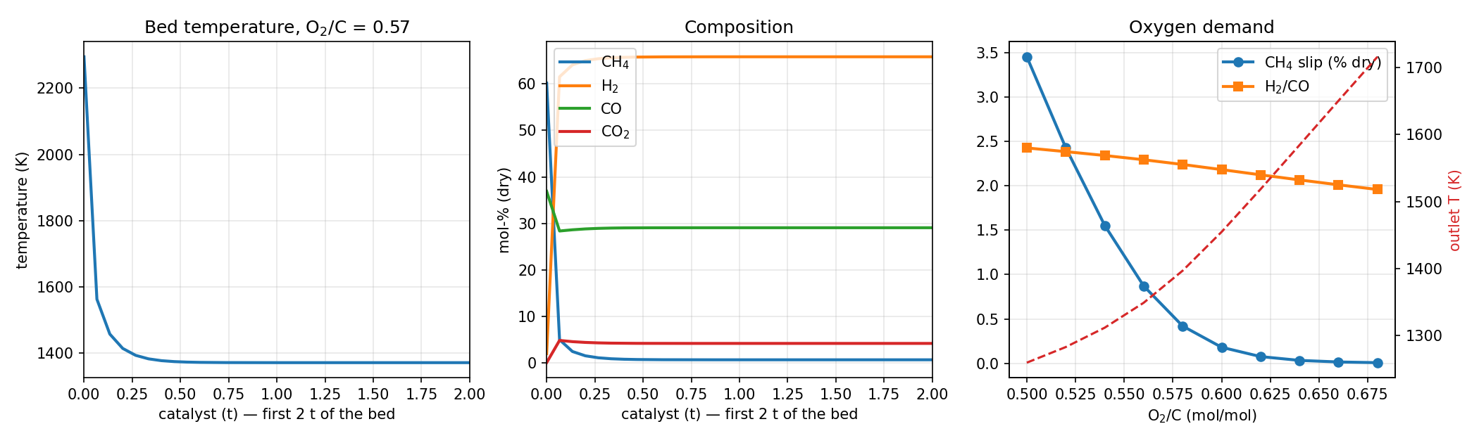
| O₂/C | Burner exit | Outlet | CH₄ slip (dry) | H₂/CO |
|---|---|---|---|---|
| 0.50 | 2 157 K | 1 260 K | 3.45 % | 2.43 |
| 0.54 | 2 237 K | 1 312 K | 1.55 % | 2.34 |
| 0.57 | 2 295 K | 1 372 K | 0.62 % | 2.27 |
| 0.60 | 2 352 K | 1 455 K | 0.18 % | 2.18 |
| 0.64 | 2 427 K | 1 584 K | 0.03 % | 2.07 |
The catalyst bed cools the gas from the flame temperature by reforming, and it reaches equilibrium within the first tonne. At these temperatures the kinetics are not limiting. The catalyst's real job is to make sure no methane or soot leaves the reactor, and the model extrapolates the Xu–Froment constants well above the range they were fitted in. The oxygen ratio then works like a thermostat. More oxygen means a hotter outlet, less methane slip and a lower H₂/CO ratio, but it costs oxygen from an air separation unit and burns valuable feed. Around O₂/C ≈ 0.55–0.6 the outlet gas has H₂/CO ≈ 2.2–2.3, close to what methanol and Fischer–Tropsch plants need. That is why large gas-to-liquids and methanol plants use autothermal reforming, alone or combined with a tubular reformer (Fiedler et al., 2000, Sec. 5.1).
"""
Steam methane reforming — autothermal reformer (ATR)
bdrworks.org · Handbook · Steam reforming, worked model 3

Heat is generated inside the reactor: oxygen burns part of the methane in a burner
zone, and the hot gas then reforms over an adiabatic nickel catalyst bed.
    burner (assumed complete, adiabatic):  CH4 + 3/2 O2 -> CO + 2 H2O
    catalyst bed (adiabatic, Xu & Froment kinetics):
        dF_i/dW = sum_j nu_ij eta_j r_j,   (sum F_i cp_i) dT/dW = sum_j (-dH_j) eta_j r_j

Run:  python atr.py      (needs numpy, scipy, matplotlib)
"""
import numpy as np
from scipy.integrate import solve_ivp
from scipy.optimize import brentq
import matplotlib.pyplot as plt

# ---------------------------------------------------------------- data
SPECIES = ["CH4", "H2O", "CO", "CO2", "H2", "N2", "O2"]
#                CH4  H2O   CO  CO2   H2  N2  O2
NU = np.array([[-1.0, -1.0, 1.0, 0.0, 3.0, 0.0, 0.0],    # 1: CH4 + H2O  <=> CO + 3 H2
               [0.0, -1.0, -1.0, 1.0, 1.0, 0.0, 0.0],    # 2: CO + H2O   <=> CO2 + H2
               [-1.0, -2.0, 0.0, 1.0, 4.0, 0.0, 0.0]])   # 3: CH4 + 2 H2O <=> CO2 + 4 H2
RG = 8.314                                                 # J/(mol K)
MW = np.array([16.043, 18.015, 28.010, 44.009, 2.016, 28.013, 31.999])   # kg/kmol

# NASA 7-coefficient polynomials (GRI-Mech 3.0 thermodynamic data): [low T < 1000 K], [high T]
NASA_LO = np.array([
    [5.14987613e+00, -1.36709788e-02, 4.91800599e-05, -4.84743026e-08, 1.66693956e-11, -1.02466476e+04, -4.64130376e+00],   # CH4
    [4.19864056e+00, -2.03643410e-03, 6.52040211e-06, -5.48797062e-09, 1.77197817e-12, -3.02937267e+04, -8.49032208e-01],   # H2O
    [3.57953347e+00, -6.10353680e-04, 1.01681433e-06, 9.07005884e-10, -9.04424499e-13, -1.43440860e+04, 3.50840928e+00],   # CO
    [2.35677352e+00, 8.98459677e-03, -7.12356269e-06, 2.45919022e-09, -1.43699548e-13, -4.83719697e+04, 9.90105222e+00],   # CO2
    [2.34433112e+00, 7.98052075e-03, -1.94781510e-05, 2.01572094e-08, -7.37611761e-12, -9.17935173e+02, 6.83010238e-01],   # H2
    [3.29867700e+00, 1.40824040e-03, -3.96322200e-06, 5.64151500e-09, -2.44485400e-12, -1.02089990e+03, 3.95037200e+00],   # N2
    [3.78245636e+00, -2.99673416e-03, 9.84730201e-06, -9.68129509e-09, 3.24372837e-12, -1.06394356e+03, 3.65767573e+00],   # O2
])
NASA_HI = np.array([
    [7.48514950e-02, 1.33909467e-02, -5.73285809e-06, 1.22292535e-09, -1.01815230e-13, -9.46834459e+03, 1.84373180e+01],   # CH4
    [3.03399249e+00, 2.17691804e-03, -1.64072518e-07, -9.70419870e-11, 1.68200992e-14, -3.00042971e+04, 4.96677010e+00],   # H2O
    [2.71518561e+00, 2.06252743e-03, -9.98825771e-07, 2.30053008e-10, -2.03647716e-14, -1.41518724e+04, 7.81868772e+00],   # CO
    [3.85746029e+00, 4.41437026e-03, -2.21481404e-06, 5.23490188e-10, -4.72084164e-14, -4.87591660e+04, 2.27163806e+00],   # CO2
    [3.33727920e+00, -4.94024731e-05, 4.99456778e-07, -1.79566394e-10, 2.00255376e-14, -9.50158922e+02, -3.20502331e+00],   # H2
    [2.92664000e+00, 1.48797680e-03, -5.68476000e-07, 1.00970380e-10, -6.75335100e-15, -9.22797700e+02, 5.98052800e+00],   # N2
    [3.28253784e+00, 1.48308754e-03, -7.57966669e-07, 2.09470555e-10, -2.16717794e-14, -1.08845772e+03, 5.45323129e+00],   # O2
])


def _a(T):
    return NASA_LO if T < 1000.0 else NASA_HI


def cp(T):
    """Ideal-gas heat capacities, J/(mol K)."""
    a = _a(T)
    return RG * (a[:, 0] + a[:, 1]*T + a[:, 2]*T**2 + a[:, 3]*T**3 + a[:, 4]*T**4)


def h(T):
    """Molar enthalpies including heats of formation, J/mol."""
    a = _a(T)
    return RG * T * (a[:, 0] + a[:, 1]*T/2 + a[:, 2]*T**2/3 + a[:, 3]*T**3/4 + a[:, 4]*T**4/5 + a[:, 5]/T)


def dH_rxn(T):
    """Heats of reactions 1-3, J/mol."""
    return NU @ h(T)


def K_eq(T):
    """Equilibrium constants of Xu & Froment: K1, K3 in bar^2, K2 dimensionless."""
    K1 = np.exp(-26830.0 / T + 30.114)
    K2 = np.exp(4400.0 / T - 4.036)
    return K1, K2, K1 * K2


def rates(T, p, eta=(1.0, 1.0, 1.0)):
    """Xu & Froment (1989) intrinsic rates times effectiveness factors, kmol/(kg_cat h); p in bar."""
    pCH4, pH2O, pCO, pCO2, pH2 = [max(x, 1e-10) for x in p[:5]]
    RT = RG * T / 1000.0                                         # kJ/mol
    k1 = 4.225e15 * np.exp(-240.1 / RT)
    k2 = 1.955e6 * np.exp(-67.13 / RT)
    k3 = 1.020e15 * np.exp(-243.9 / RT)
    KCO = 8.23e-5 * np.exp(70.65 / RT)
    KH2 = 6.12e-9 * np.exp(82.90 / RT)
    KCH4 = 6.65e-4 * np.exp(38.28 / RT)
    KH2O = 1.77e5 * np.exp(-88.68 / RT)
    K1, K2, K3 = K_eq(T)
    den = 1.0 + KCO*pCO + KH2*pH2 + KCH4*pCH4 + KH2O*pH2O/pH2
    r1 = k1 / pH2**2.5 * (pCH4*pH2O - pH2**3*pCO/K1) / den**2
    r2 = k2 / pH2 * (pCO*pH2O - pH2*pCO2/K2) / den**2
    r3 = k3 / pH2**3.5 * (pCH4*pH2O**2 - pH2**4*pCO2/K3) / den**2
    return np.array([eta[0]*r1, eta[1]*r2, eta[2]*r3])


def equilibrium(T, P, n0):
    """Equilibrium of reactions 1 and 2 (3 is their sum) from flows n0 at T (K), P (bar)."""
    from scipy.optimize import fsolve
    K1, K2, _ = K_eq(T)
    def res(x):
        n = np.maximum(n0 + NU[0]*x[0] + NU[1]*x[1], 1e-14)
        p = P * n / n.sum()
        return [np.log(p[2]*p[4]**3 / (p[0]*p[1])) - np.log(K1), np.log(p[3]*p[4] / (p[2]*p[1])) - np.log(K2)]
    x = fsolve(res, [0.7*n0[0], 0.2*n0[0]], xtol=1e-12)
    return n0 + NU[0]*x[0] + NU[1]*x[1]


# ---------------------------------------------------------------- ATR
P = 30.0                              # bar
F_CH4 = 1000.0                        # natural gas (as CH4), kmol/h
S_C = 0.6                             # steam-to-carbon ratio (low, as in modern ATRs)
T_GAS, T_O2 = 900.0, 500.0            # preheat of CH4 + steam, and of the oxygen, K
W_CAT = 20e3                          # catalyst, kg
ETA = (0.03, 0.03, 0.03)
BURN = np.array([-1.0, 2.0, 1.0, 0.0, 0.0, 0.0, -1.5])     # CH4 + 1.5 O2 -> CO + 2 H2O


def burner(o2_c):
    """Adiabatic flame: all O2 burns CH4 to CO + H2O. Returns flows (kmol/h) and temperature (K)."""
    gas = np.array([F_CH4, S_C * F_CH4, 0, 0, 0.02 * F_CH4, 0.01 * F_CH4, 0])
    o2 = np.zeros(7); o2[6] = o2_c * F_CH4
    H_in = np.dot(gas, h(T_GAS)) + np.dot(o2, h(T_O2))
    n = gas + o2 + BURN * (o2_c * F_CH4 / 1.5)
    T = brentq(lambda T: np.dot(n, h(T)) - H_in, 600, 4000)
    return n, T


def rhs(W, u):
    F, T = u[:7], u[7]
    r = rates(T, P * F / F.sum(), ETA)                       # kmol/(kg h)
    return np.append(NU.T @ r, np.dot(-dH_rxn(T), r) * 1e3 / np.dot(F * 1e3, cp(T)))


def atr(o2_c, n=300):
    n0, Tb = burner(o2_c)
    sol = solve_ivp(rhs, (0, W_CAT), np.append(n0, Tb), method="LSODA", rtol=1e-8, atol=1e-8, dense_output=True)
    w = np.linspace(0, W_CAT, n)
    return w, sol.sol(w), Tb


def summary(u):
    F = u[:7, -1]
    return dict(T=u[7, -1], X=1 - F[0] / F_CH4, slip=100 * F[0] / (F.sum() - F[1]), h2co=F[4] / F[2],
                syngas=F[4] + F[2])


if __name__ == "__main__":
    o2c = 0.57
    w, u, Tb = atr(o2c)
    s = summary(u)
    ne = equilibrium(s["T"], P, u[:7, 0])
    print(f"ATR {P:.0f} bar, S/C {S_C}, O2/C {o2c}: burner exit {Tb:.0f} K, bed outlet {s['T']:.0f} K")
    print(f"CH4 conversion {100*s['X']:.1f} % (equilibrium at outlet {100*(1-ne[0]/F_CH4):.1f} %), "
          f"slip {s['slip']:.2f} % dry, H2/CO {s['h2co']:.2f}, H2+CO {s['syngas']:.0f} kmol/h")

    o2s = np.arange(0.50, 0.681, 0.02)
    rows = [summary(atr(x, 60)[1]) for x in o2s]
    for x, r in zip(o2s, rows):
        print(f"  O2/C {x:.2f}: outlet {r['T']:.0f} K, slip {r['slip']:.2f} %, H2/CO {r['h2co']:.2f}")

    fig, ax = plt.subplots(1, 3, figsize=(14, 4.2))
    ax[0].plot(w / 1e3, u[7], lw=2); ax[0].set(xlabel="catalyst (t)", ylabel="temperature (K)", title=f"Bed temperature, O$_2$/C = {o2c}")
    dry = u[:7].sum(axis=0) - u[1]
    for i, lab in [(0, "CH$_4$"), (4, "H$_2$"), (2, "CO"), (3, "CO$_2$")]:
        ax[1].plot(w / 1e3, 100 * u[i] / dry, lw=2, label=lab)
    ax[1].set(xlabel="catalyst (t)", ylabel="mol-% (dry)", title="Composition"); ax[1].legend()
    ax[2].plot(o2s, [r["slip"] for r in rows], "o-", lw=2, label="CH$_4$ slip (% dry)")
    ax[2].plot(o2s, [r["h2co"] for r in rows], "s-", lw=2, label="H$_2$/CO")
    ax[2].set(xlabel="O$_2$/C (mol/mol)", title="Oxygen demand"); ax[2].legend()
    a2 = ax[2].twinx(); a2.plot(o2s, [r["T"] for r in rows], "--", c="C3"); a2.set_ylabel("outlet T (K)", color="C3")
    for a in ax[:2]:
        a.set_xlim(0, 2)                                   # equilibrium is reached in the first tonnes
    ax[0].set_xlabel("catalyst (t) — first 2 t of the bed"); ax[1].set_xlabel("catalyst (t) — first 2 t of the bed")
    for a in ax:
        a.grid(alpha=0.3)
    fig.tight_layout(); fig.savefig("atr.png", dpi=150)
    plt.show()
function atr()
% Steam methane reforming - autothermal reformer (burner + adiabatic Ni bed)
% bdrworks.org - Handbook - Steam reforming, worked model 3
% Save as atr.m and run:  atr

p.P = 30; p.F = 1000; p.SC = 0.6; p.Tg = 900; p.To2 = 500; p.W = 20e3; p.eta = [0.03 0.03 0.03];
for o2c = [0.50 0.54 0.57 0.60 0.64]
    [n0, Tb] = burner(o2c, p);
    opts = odeset('RelTol', 1e-8, 'AbsTol', 1e-8);
    [~, u] = ode45(@(W,u) bed(u, p), [0 p.W], [n0; Tb], opts);
    F = u(end,1:7)';  dry = sum(F) - F(2);
    fprintf('O2/C %.2f: burner %.0f K, outlet %.0f K, CH4 slip %.2f %% dry, H2/CO %.2f\n', o2c, Tb, u(end,8), 100*F(1)/dry, F(5)/F(3));
end
end

function [n, T] = burner(o2c, p)
gas = [p.F; p.SC*p.F; 0; 0; 0.02*p.F; 0.01*p.F; 0];  o2 = [0; 0; 0; 0; 0; 0; o2c*p.F];
Hin = gas'*h_all(p.Tg) + o2'*h_all(p.To2);
n = gas + o2 + [-1; 2; 1; 0; 0; 0; -1.5]*(o2c*p.F/1.5);    % CH4 + 1.5 O2 -> CO + 2 H2O
T = fzero(@(T) n'*h_all(T) - Hin, [600 4000]);
end

function du = bed(u, p)
F = u(1:7);  T = u(8);  nu = stoich();
r = rates(T, p.P*F/sum(F), p.eta);                        % kmol/(kg h)
du = [nu'*r; (-dH_rxn(T))'*r/(F'*cp_all(T))];
end

% ================================================================ properties & kinetics
function nu = stoich()
%       CH4 H2O  CO CO2  H2 N2  O2
nu = [  -1  -1    1   0   3  0   0;      % CH4 + H2O   <=> CO + 3H2
         0  -1   -1   1   1  0   0;      % CO + H2O    <=> CO2 + H2
        -1  -2    0   1   4  0   0];     % CH4 + 2H2O  <=> CO2 + 4H2
end

function a = nasa(T)
% NASA 7-coefficient polynomials (GRI-Mech 3.0) for CH4 H2O CO CO2 H2 N2 O2
if T < 1000
  a = [
     5.14987613e+00, -1.36709788e-02, 4.91800599e-05, -4.84743026e-08, 1.66693956e-11, -1.02466476e+04, -4.64130376e+00;   % CH4
     4.19864056e+00, -2.03643410e-03, 6.52040211e-06, -5.48797062e-09, 1.77197817e-12, -3.02937267e+04, -8.49032208e-01;   % H2O
     3.57953347e+00, -6.10353680e-04, 1.01681433e-06, 9.07005884e-10, -9.04424499e-13, -1.43440860e+04, 3.50840928e+00;   % CO
     2.35677352e+00, 8.98459677e-03, -7.12356269e-06, 2.45919022e-09, -1.43699548e-13, -4.83719697e+04, 9.90105222e+00;   % CO2
     2.34433112e+00, 7.98052075e-03, -1.94781510e-05, 2.01572094e-08, -7.37611761e-12, -9.17935173e+02, 6.83010238e-01;   % H2
     3.29867700e+00, 1.40824040e-03, -3.96322200e-06, 5.64151500e-09, -2.44485400e-12, -1.02089990e+03, 3.95037200e+00;   % N2
     3.78245636e+00, -2.99673416e-03, 9.84730201e-06, -9.68129509e-09, 3.24372837e-12, -1.06394356e+03, 3.65767573e+00;   % O2
  ];
else
  a = [
     7.48514950e-02, 1.33909467e-02, -5.73285809e-06, 1.22292535e-09, -1.01815230e-13, -9.46834459e+03, 1.84373180e+01;   % CH4
     3.03399249e+00, 2.17691804e-03, -1.64072518e-07, -9.70419870e-11, 1.68200992e-14, -3.00042971e+04, 4.96677010e+00;   % H2O
     2.71518561e+00, 2.06252743e-03, -9.98825771e-07, 2.30053008e-10, -2.03647716e-14, -1.41518724e+04, 7.81868772e+00;   % CO
     3.85746029e+00, 4.41437026e-03, -2.21481404e-06, 5.23490188e-10, -4.72084164e-14, -4.87591660e+04, 2.27163806e+00;   % CO2
     3.33727920e+00, -4.94024731e-05, 4.99456778e-07, -1.79566394e-10, 2.00255376e-14, -9.50158922e+02, -3.20502331e+00;   % H2
     2.92664000e+00, 1.48797680e-03, -5.68476000e-07, 1.00970380e-10, -6.75335100e-15, -9.22797700e+02, 5.98052800e+00;   % N2
     3.28253784e+00, 1.48308754e-03, -7.57966669e-07, 2.09470555e-10, -2.16717794e-14, -1.08845772e+03, 5.45323129e+00;   % O2
  ];
end
end

function c = cp_all(T)
a = nasa(T);  c = 8.314*(a(:,1) + a(:,2)*T + a(:,3)*T^2 + a(:,4)*T^3 + a(:,5)*T^4);     % J/(mol K)
end

function H = h_all(T)
a = nasa(T);  H = 8.314*T*(a(:,1) + a(:,2)*T/2 + a(:,3)*T^2/3 + a(:,4)*T^3/4 + a(:,5)*T^4/5 + a(:,6)/T);   % J/mol
end

function dH = dH_rxn(T)
dH = stoich()*h_all(T);
end

function [K1, K2, K3] = K_eq(T)
K1 = exp(-26830/T + 30.114);  K2 = exp(4400/T - 4.036);  K3 = K1*K2;      % Xu & Froment
end

function r = rates(T, p, eta)
% Xu & Froment (1989) rates times effectiveness factors, kmol/(kg_cat h); p in bar [CH4 H2O CO CO2 H2 ...]
p = max(p, 1e-10);  RT = 8.314e-3*T;
k1 = 4.225e15*exp(-240.1/RT);  k2 = 1.955e6*exp(-67.13/RT);  k3 = 1.020e15*exp(-243.9/RT);
KCO = 8.23e-5*exp(70.65/RT);  KH2 = 6.12e-9*exp(82.90/RT);  KCH4 = 6.65e-4*exp(38.28/RT);  KH2O = 1.77e5*exp(-88.68/RT);
[K1, K2, K3] = K_eq(T);
den = 1 + KCO*p(3) + KH2*p(5) + KCH4*p(1) + KH2O*p(2)/p(5);
r = eta(:).*[k1/p(5)^2.5*(p(1)*p(2) - p(5)^3*p(3)/K1)/den^2;
             k2/p(5)*(p(3)*p(2) - p(5)*p(4)/K2)/den^2;
             k3/p(5)^3.5*(p(1)*p(2)^2 - p(5)^4*p(4)/K3)/den^2];
end

function n = equilibrium(T, P, n0)
% equilibrium of reactions 1 and 2 by Newton's method on the log equations
nu = stoich();  [K1, K2] = K_eq(T);  x = [0.7*n0(1); 0.2*n0(1)];
f = @(x) eqres(x, n0, nu, P, K1, K2);
for it = 1:100
    F = f(x);  J = zeros(2);  h = 1e-7*max(abs(x), 1e-6);
    for j = 1:2, e = zeros(2,1); e(j) = h(j); J(:,j) = (f(x + e) - F)/h(j); end
    dx = -J\F;  lam = 1;
    while any(n0 + nu(1,:)'*(x(1)+lam*dx(1)) + nu(2,:)'*(x(2)+lam*dx(2)) < 0 & [1 1 1 1 1 0 0]') && lam > 1e-4, lam = lam/2; end
    x = x + lam*dx;
    if norm(dx) < 1e-12*max(1, norm(x)), break; end
end
n = n0 + nu(1,:)'*x(1) + nu(2,:)'*x(2);
end

function F = eqres(x, n0, nu, P, K1, K2)
n = max(n0 + nu(1,:)'*x(1) + nu(2,:)'*x(2), 1e-14);  p = P*n/sum(n);
F = [log(p(3)*p(5)^3/(p(1)*p(2))) - log(K1);  log(p(4)*p(5)/(p(3)*p(2))) - log(K2)];
end
7Comparison
| Fired tubular reformer (S/C 3) | Autothermal reformer (S/C 0.6) | |
|---|---|---|
| Heat supply | External, through the tube wall | Internal, combustion with O₂ |
| Outlet temperature | ≈ 1 120 K | ≈ 1 300–1 400 K |
| CH₄ slip (dry) | ≈ 7 % | < 1 % |
| H₂/CO | ≈ 5.7 (good for H₂, NH₃) | ≈ 2.2–2.3 (good for MeOH, FT) |
| Limiting factor | Tube-metal temperature | Oxygen cost, soot, refractory |
| Typical use | Hydrogen, ammonia, small methanol plants | Large methanol and GTL plants |
The two technologies are also combined. In ammonia plants a primary tubular reformer is followed by an air-blown secondary reformer, which supplies the nitrogen at the same time (Appl, 2000, Sec. 4.5.1.1). Newer concepts replace the fired primary reformer by an exchanger reformer heated by the hot secondary-reformer effluent (Appl, 2000, Sec. 4.5.1.1). In "combined reforming" for methanol, only part of the natural gas is steam reformed, and the remainder passes with the reformed gas through an autothermal reformer, so that the mixed gas reaches the stoichiometric number the loop needs (Fiedler et al., 2000, Sec. 5.1).
8Try it
Both reactors, ported to JavaScript with the same kinetics and thermodynamics, run below. Try firing the tube harder until the wall passes 1 230 K, or lowering the steam ratio.
9Going further
- Replace the prescribed heat flux with a furnace model. A simple well-stirred furnace with radiative exchange to the tube wall already predicts the flux profile.
- Add a carbon-formation check: compare the local pCH₄/pH₂² with the equilibrium of methane cracking along the tube, and find the lowest safe S/C.
- Compute pellet effectiveness factors from a diffusion–reaction model instead of fixing η = 0.03, and see where along the tube the assumption fails.
- Model an air-blown secondary reformer after the tubular reformer and adjust the air flow to reach H₂/N₂ = 3 for a synthesis gas.
- Mix the outputs of a tubular reformer and an ATR to reach SN = 2.05 for the methanol loop.
10References
- Appl, M. (2000). Ammonia. In Ullmann's Encyclopedia of Industrial Chemistry. Wiley-VCH, Weinheim. doi:10.1002/14356007.a02_143
- Brent, R. P. (1973). Algorithms for Minimization without Derivatives. Prentice-Hall, Englewood Cliffs, NJ.
- Ergun, S. (1952). Fluid flow through packed columns. Chem. Eng. Prog., 48(2), 89–94.
- Fiedler, E., Grossmann, G., Kersebohm, D. B., Weiss, G., & Witte, C. (2000). Methanol. In Ullmann's Encyclopedia of Industrial Chemistry. Wiley-VCH, Weinheim. doi:10.1002/14356007.a16_465
- Finlayson, B. A., Biegler, L. T., & Grossmann, I. E. (2006). Mathematics in chemical engineering. In Ullmann's Encyclopedia of Industrial Chemistry. Wiley-VCH, Weinheim. doi:10.1002/14356007.b01_01.pub2
- Froment, G. F., Bischoff, K. B., & De Wilde, J. (2011). Chemical Reactor Analysis and Design (3rd ed.). Wiley, Hoboken, NJ.
- Goodwin, D. G., Speth, R. L., Moffat, H. K., & Weber, B. W. (2023). Cantera: An object-oriented software toolkit for chemical kinetics, thermodynamics, and transport processes. https://www.cantera.org.
- Gordon, S., & McBride, B. J. (1994). Computer Program for Calculation of Complex Chemical Equilibrium Compositions and Applications (CEA), Part I: Analysis. NASA Reference Publication 1311, Cleveland, OH.
- Leva, M. (1947). Heat transfer to gases through packed tubes. Ind. Eng. Chem., 39, 857–862.
- Rostrup-Nielsen, J. R. (1984). Catalytic steam reforming. In Catalysis: Science and Technology, Vol. 5 (Anderson, J. R., Boudart, M., Eds.). Springer, Berlin.
- Smith, G. P., Golden, D. M., Frenklach, M., Moriarty, N. W., Eiteneer, B., Goldenberg, M., Bowman, C. T., Hanson, R. K., Song, S., Gardiner, W. C., Lissianski, V. V., & Qin, Z. (1999). GRI-Mech 3.0 (thermodynamic data, NASA polynomials). Gas Research Institute, http://combustion.berkeley.edu/gri-mech/.
- Xu, J., & Froment, G. F. (1989a). Methane steam reforming, methanation and water-gas shift: I. Intrinsic kinetics. AIChE J., 35(1), 88–96.
- Xu, J., & Froment, G. F. (1989b). Methane steam reforming: II. Diffusional limitations and reactor simulation. AIChE J., 35(1), 97–103.
Tube dimensions, heat-flux profile, effectiveness factor and ATR conditions are round numbers chosen for teaching, not data from a specific plant. The kinetic and thermodynamic data are from the open literature cited above.