Research article · Adsorption & thermal imaging

Thermal imaging and 2D modelling of the adsorption heat front in a 13X zeolite bed drying a hydrogen-rich gas

bdrworks.org · 24 September 2026

Figure 1. Graphical abstract. Thermal image of the bed at 17:47 with the axial temperature rise along the tube: measured from the image pixels (white) and predicted by the 2D model for the outer wall surface (dashed blue). Gas enters from the top.

Abstract

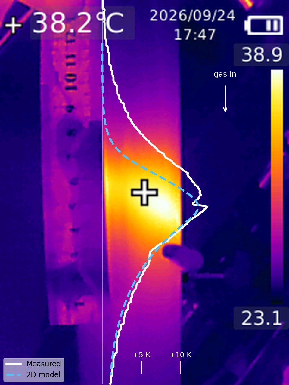
A hydrogen–nitrogen stream saturated with water at 22 °C and diluted with helium was passed down a 22 cm bed of 2 mm 13X zeolite beads in an acrylic tube. The heat of adsorption produced a travelling hot band, which was recorded with a handheld thermal camera. The camera images were converted to temperature maps by matching every pixel to the colour scale of the image. The axial surface-temperature profile was then compared with a transient, two-dimensional (r–z) non-isothermal adsorption model. Every transport property in the model was calculated from standard correlations for this gas and packing. Only the linear driving force constant and the outer heat transfer coefficient were fitted to one image. The model reproduces the measured profile with an RMS error of 0.86 K, and the peak temperature rise within 1.4 K. The fitted outer coefficient (8.5 W/m²K) lies within 10 % of the Churchill–Chu correlation with radiation. The profile is asymmetric, steep upstream and exponentially decaying downstream, because the thermal wave travels about 20 times faster than the adsorption front. The measured downstream decay length is 3.5 cm against 3.3 cm from the model. The model also predicts that the bed centre is about 13 K hotter than the wall seen by the camera.

Keywords zeolite 13X · water adsorption · fixed bed · thermal wave · infrared thermography · LDF model

Highlights

The adsorption heat front in a 13X drier was imaged with a low-cost thermal camera and converted pixel by pixel to temperature.
A 2D r–z model built from literature correlations fits the wall profile to 0.9 K with only two fitted parameters.
The asymmetric band shape follows from a thermal wave that outruns the concentration front by a factor of about 20.
The camera sees the acrylic surface; the model puts the bed centre about 13 K hotter.

1. Introduction

Zeolite 13X is one of the standard adsorbents for drying gases. It is a sodium X zeolite with large cavities and strong cation sites. It takes up water from very low partial pressures to roughly a quarter of its own mass (Breck, 1974; Roland & Kleinschmit, 2000). Because the heat of adsorption of water is large, well above the heat of condensation at low loading, a drying bed does not stay isothermal (Ruthven, 1984). Water is removed in a narrow mass-transfer zone that moves slowly along the column. Upstream of it the zeolite is saturated; downstream it is still dry (Ruthven, 1984; Seader et al., 2011). The heat released in this zone travels with the gas and forms a temperature front.

The interaction of this thermal front with the concentration front is a classical problem in fixed-bed adsorption. When the heat capacity of the gas flow is large compared with the rate at which the front advances, the heat released is pushed ahead of the adsorption zone and a "pure thermal wave" forms (Pan & Basmadjian, 1970). In small laboratory columns the wall loses much of this heat. The measured temperatures then depend strongly on the wall and its surroundings.

Temperatures in adsorption columns are usually measured with a few thermocouples. A thermal camera gives the whole axial profile of the wall at once, but it measures the outer surface of the wall, not the packing, and the reading depends on emissivity, view angle and reflections (Vollmer & Möllmann, 2017). This work has three aims: to extract a quantitative temperature profile from ordinary thermal camera images of a working 13X bed; to compare it with a 2D model whose inputs come from the literature; and to find out what the camera does and does not tell about the temperature inside the bed.

2. Experimental

2.1 Set-up

A mixture of 900 sccm H₂ and 300 sccm N₂ was passed through an acid trap and saturated with water at a room temperature of 22 °C. It was then mixed with 200 sccm He and fed to the top of the zeolite bed (Table 1). The bed was a 22 cm packed length of 13X beads with a mean diameter of about 2 mm, activated beforehand at 250 °C in a furnace. It was held in an acrylic tube of 50 mm outer and 42 mm inner diameter. The flow had been changed during earlier tests, so the upper part of the bed was already partly saturated, and the hot band was observed near the middle of the column.

Quantity	Value
Feed	900 sccm H₂ + 300 sccm N₂, water-saturated at 22 °C, + 200 sccm He
Water in the feed	32.1 sccm, 2.24 mol % (p = 2.27 kPa)
Superficial velocity, particle Reynolds number	1.71 cm/s, Re = 0.75
Adsorbent	13X zeolite beads, d_p ≈ 2 mm, activated at 250 °C
Column	Acrylic, 50 mm OD / 42 mm ID, 22 cm packed length, D/d_p = 21, downflow
Camera	Handheld thermal camera, 240 × 320 px, ironbow palette, auto-ranged scale

Table 1. Operating conditions. Standard volumes refer to 25 °C and 1 atm.

2.2 Thermal images

Four images were taken between 17:36 and 17:48 (Figure 2): one of the whole bed, one close-up, and two blended visible/thermal views with a ruler held beside the tube. The camera scales its palette to the minimum and maximum temperature of each frame and prints both values on the image.

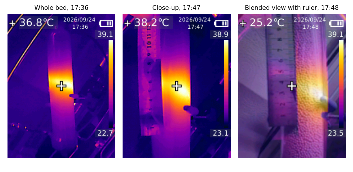
Three thermal camera images of the zeolite column. — **Figure 2.** Thermal images of the column: (a) whole bed, 17:36; (b) close-up, 17:47; (c) blended visible/thermal view with a ruler, 17:48.

2.3 Image-to-temperature conversion

The colour bar of each image was read column by column, and each bar pixel was assigned a temperature linearly between the printed minimum and maximum. Every image pixel was then given the temperature of the nearest bar colour in RGB space; with the camera's own palette the match was exact. The axial profile is the median over the central strip of the tube, with the cursor and the side fitting masked. Only the pure thermal images were used quantitatively, because blending with the visible image changes the colours.

Acrylic is practically opaque in the 8–14 µm band and has a high emissivity, so the camera reads the outer wall surface. Emissivity falls at grazing view angles, which makes the edges of the cylinder appear cooler (Vollmer & Möllmann, 2017). Axial distances were scaled from the 50 mm outer diameter of the tube (11.0 and 12.6 px/cm). The ruler stood closer to the camera than the tube and appeared about 1.6 times larger, so it was used only to locate the band. Temperatures are reported as the rise above the image background, which the camera read at 24.2 °C against a room temperature of 22 °C.

3. Model

3.1 Governing equations

The column is treated as a transient, non-isothermal fixed-bed adsorber with axial symmetry (Ruthven, 1984; Froment et al., 2011, Ch. 11). The model rests on five assumptions:

water is dilute (2.2 mol %), so the gas velocity is constant;
gas and solid are in local thermal equilibrium;
uptake follows the linear driving force approximation;
the pressure drop is negligible, a few pascals by the Ergun equation (Ergun, 1952);
the acrylic wall is resolved as a separate conducting domain.

The water balance in the gas phase is

$$\varepsilon\frac{\partial c}{\partial t} = -u\frac{\partial c}{\partial z} + \varepsilon D_{ax}\frac{\partial^2 c}{\partial z^2} + \varepsilon D_r \frac{1}{r}\frac{\partial}{\partial r}\!\left(r\frac{\partial c}{\partial r}\right) - \rho_b\frac{\partial q}{\partial t} \tag{1}$$

The uptake rate follows the linear driving force (LDF) model (Glueckauf, 1955; Sircar & Hufton, 2000):

$$\frac{\partial q}{\partial t} = k_{LDF}\,\big(q^*(p,T) - q\big) \tag{2}$$

Equilibrium is described by a temperature-dependent Langmuir isotherm (Ruthven, 1984):

$$q^* = \frac{q_m\, b\, p}{1 + b\, p}, \qquad b = b_0 \exp\!\left(\frac{Q}{RT}\right) \tag{3}$$

The energy balance of the pseudo-homogeneous bed includes the heat capacity of the adsorbed water and the heat of adsorption as a source (Ruthven, 1984; Froment et al., 2011, Ch. 11):

$$\begin{aligned}\left(\rho_b c_s + \rho_b q M_w c_l\right)\frac{\partial T}{\partial t} ={}& -G c_p\frac{\partial T}{\partial z} + k_{ax}\frac{\partial^2 T}{\partial z^2} \\ &+ k_r\frac{1}{r}\frac{\partial}{\partial r}\!\left(r\frac{\partial T}{\partial r}\right) + \rho_b(-\Delta H)\frac{\partial q}{\partial t}\end{aligned} \tag{4}$$

In the acrylic wall only conduction acts, radially and axially:

$$\rho_w c_{p,w}\frac{\partial T_w}{\partial t} = k_w\left[\frac{1}{r}\frac{\partial}{\partial r}\!\left(r\frac{\partial T_w}{\partial r}\right) + \frac{\partial^2 T_w}{\partial z^2}\right] \tag{5}$$

3.2 Boundary and initial conditions

At the inlet, Danckwerts conditions are applied; the outlet has zero gradients (Danckwerts, 1953). The axis is a symmetry line. Heat passes from the packing to the wall and from the wall to the room through

$$\begin{aligned} -k_r\left.\frac{\partial T}{\partial r}\right|_{R_i} &= h_w\,(T - T_{w})\big|_{R_i} \\ -k_w\left.\frac{\partial T_w}{\partial r}\right|_{R_o} &= h_o\,(T_{w} - T_\infty)\big|_{R_o} \end{aligned} \tag{6}$$

To represent the partly saturated bed, the first 8 cm were initialised at equilibrium with the feed and the rest dry, all at 22 °C. The comparison uses the profile shape after 3 h, when a constant pattern has formed.

3.3 Parameters

All physical and transport properties were calculated for this gas mixture and packing (Table 2). Only k_LDF and h_o were fitted, by minimising the RMS difference between the peak-aligned model and measured profiles of the whole-bed image over −7 to +9 cm. The fit used a grid of 3 × 4 values.

Quantity	Value	Source
Water vapour pressure at 22 °C	2.64 kPa	Magnus form (Alduchov & Eskridge, 1996); agrees with IAPWS-IF97 (2.64 kPa) (IAPWS, 2012)
Water in feed	32.1 sccm, y = 2.24 %	Saturation assumed complete; sccm at 25 °C, 1 atm
Gas heat capacity	27.9 J/mol·K	Ideal-gas values at 298 K (NIST, 2023)
Gas viscosity	15.3 µPa·s	Pure gases (NIST, 2023; Huber et al., 2009), mixed with Wilke's rule (Wilke, 1950)
Gas thermal conductivity	0.121 W/m·K	Pure gases (NIST, 2023; Huber et al., 2012), Wassiljewa form with Mason–Saxena coefficients (Mason & Saxena, 1958; Poling et al., 2001, Ch. 10)
H₂O diffusivity in the mix	5.74 × 10⁻⁵ m²/s	Binary pairs (Fuller et al., 1966), Blanc's law for the mixture (Poling et al., 2001, Ch. 11)
Superficial velocity, Re, Pr	1.71 cm/s, 0.75, 0.43	From the feed; Re based on d_p
Bed voidage ε	0.403	Spheres at D/d_p = 21 (Dixon, 1988)
Bulk density ρ_b	680 kg/m³	Typical commercial 13X beads (Roland & Kleinschmit, 2000) (assumed; see note below)
Solid heat capacity c_s	920 J/kg·K	Assumed, typical for dehydrated aluminosilicates
Adsorbed water heat capacity c_l	4180 J/kg·K	Taken as liquid water (IAPWS, 2012)
Isotherm q_m, b(298 K), Q	15.5 mol/kg; 0.10 Pa⁻¹; 50 kJ/mol	Steep type I shape and a capacity near 0.28 g/g, as reported for 13X (Breck, 1974; Wang & LeVan, 2009)
Heat of adsorption −ΔH	52 kJ/mol	Between the heat of condensation, 44 kJ/mol (IAPWS, 2012), and the higher values at low loading (Breck, 1974; Ruthven, 1984)
Axial dispersion D_ax	4.75 × 10⁻⁵ m²/s	Gas dispersion correlation (Edwards & Richardson, 1968)
Radial dispersion D_r	4.96 × 10⁻⁵ m²/s	Molecular term plus Pe_r,∞ ≈ 11 (Froment et al., 2011, Ch. 11)
Stagnant bed conductivity k_e0	0.163 W/m·K	Zehner–Schlünder model (Zehner & Schlünder, 1970; VDI, 2010) with particle conductivity 0.2 W/m·K (assumed)
Radial / axial conductivity k_r, k_ax	0.168 / 0.183 W/m·K	k_e0 + G c_p d_p/8 (Martin & Nilles, 1993) and + G c_p d_p/2 (Yagi et al., 1960)
Bed-to-wall coefficient h_w	133 W/m²K	Nu_w = (1.3 + 5 d_p/D) k_e0/k_g + 0.19 Re^0.75 Pr^1/3 (Martin & Nilles, 1993; VDI, 2010)
Acrylic wall k_w, ρc_p	0.19 W/m·K; 1.75 MJ/m³K	PMMA property data (Mark, 1999)
Outer coefficient h_o, correlation	3.8 + 5.6 = 9.4 W/m²K	Natural convection (Churchill & Chu, 1975a) plus linearised radiation with ε = 0.9 (Bergman et al., 2011; Vollmer & Möllmann, 2017)
Outer coefficient h_o, fitted	8.5 W/m²K	Fitted to the whole-bed image; 10 % below the correlation
LDF constant k_LDF, estimate	5.3 × 10⁻³ s⁻¹	Macropore diffusion, k = 15 ε_pD_pc₀/(R_p²ρ_pq₀) (Glueckauf, 1955; Ruthven, 1984), ε_p = 0.35, τ = 3 (assumed)
LDF constant k_LDF, fitted	1.0 × 10⁻⁴ s⁻¹	Fitted to the whole-bed image (an effective value, see below)

Table 2. Model inputs. Every value is either calculated from the cited correlation for these conditions, taken from a data source, fitted, or marked as assumed.

3.4 Numerical solution

Equations (1)–(6) were discretised with finite volumes into 110 axial × 6 radial cells in the bed and 3 radial cells in the wall, about 2300 ordinary differential equations. The system was solved as a method-of-lines problem (Finlayson et al., 2006) with SciPy's variable-order BDF integrator and a sparse Jacobian pattern (Virtanen et al., 2020; Shampine & Reichelt, 1997). One 3 h simulation takes a few seconds to about a minute.

4. Results and discussion

4.1 Axial temperature profile

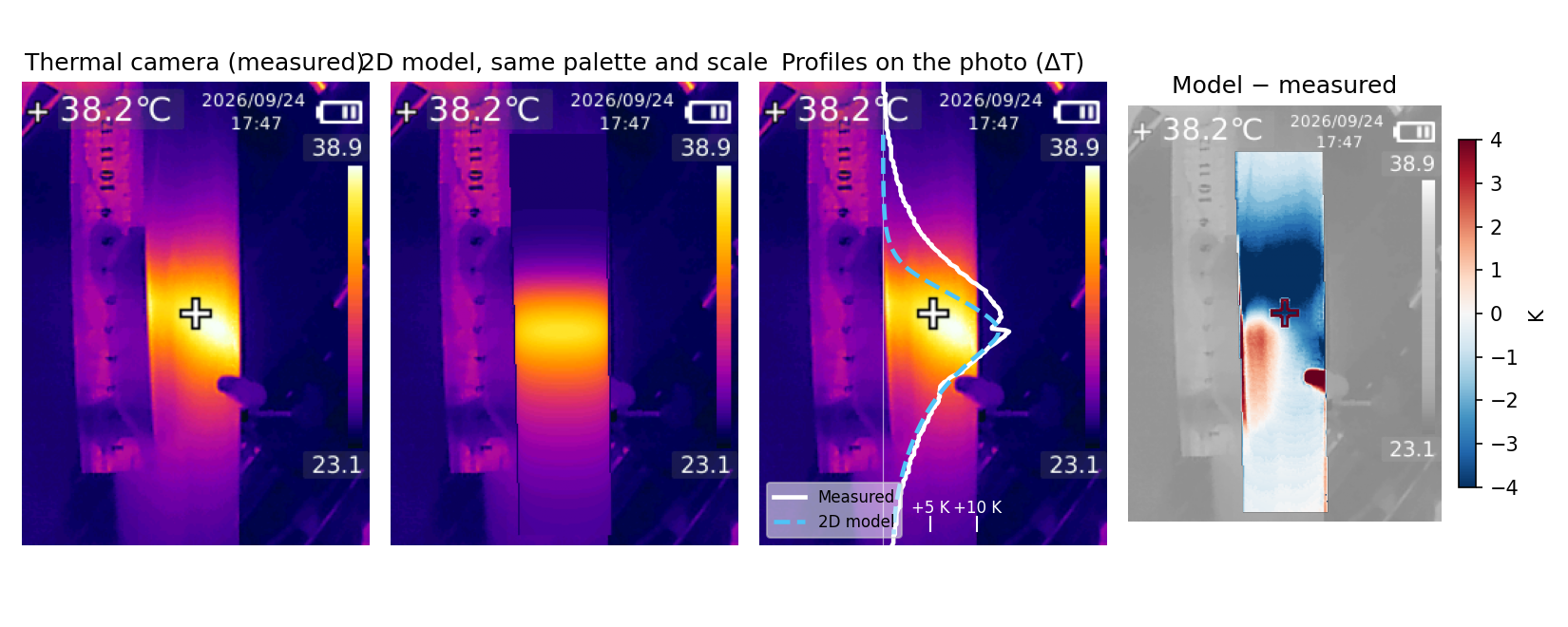
Figure 3 compares the peak-aligned profiles. With the fitted k_LDF = 1.0 × 10⁻⁴ s⁻¹ and h_o = 8.5 W/m²K, the model follows the whole-bed image with an RMS error of 0.86 K (Table 3). The downstream tail agrees closely in both images. The close-up taken 11 minutes later is wider on the upstream side, which raises its RMS error to 2.4 K.

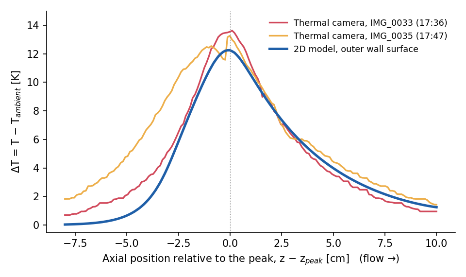
Measured and modelled temperature rise along the bed, aligned at the peak. — **Figure 3.** Temperature rise of the outer wall surface along the tube, aligned at the peak: two thermal images and the 2D model (t = 3 h).

Quantity	Image, 17:36	Image, 17:47	Model
Peak rise ΔT_max [K]	13.6	13.3	12.2
Half width, upstream [cm]	2.4	4.1	2.4
Half width, downstream [cm]	2.7	2.6	3.2
Downstream decay length [cm]	3.5	–	3.3
RMS error of the profile [K]	0.86	2.37	–
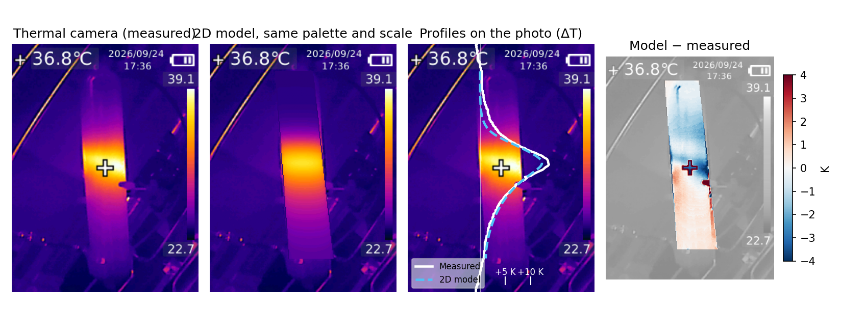
RMS error, pixel by pixel [K]	1.8	2.6	–

Table 3. Measured and modelled profile metrics. Half widths are measured from the peak to half of ΔT_max.

4.2 Pixel-level comparison

The model surface temperature was also painted back onto each photograph with the camera's own palette and scale, and the difference was mapped pixel by pixel (Figures 4 and 5). In the difference map the upstream side is blue (model cooler) and the downstream side slightly red. The real front is therefore broader upstream and decays a little faster downstream than the model. In the close-up the hot region also leans towards one side of the tube, which an axisymmetric model cannot produce.

Measured thermal image, model in the same palette, profiles on the photo, and difference map for the whole-bed image. — **Figure 4.** Whole-bed image, 17:36: (a) measurement; (b) model rendered in the same palette and scale; (c) both profiles drawn on the photograph; (d) model minus measurement.

The same four-panel comparison for the close-up image. — **Figure 5.** The same comparison for the close-up, 17:47.

4.3 Shape of the thermal front

The asymmetric profile follows from the ratio of two velocities. The thermal wave moves at

$$u_T = \frac{G c_p}{\rho_b c_s} \approx 11\ \text{cm/h} \tag{7}$$

while the adsorption front moves at only u_c ≈ 0.54 cm/h. Because u_T ≫ u_c, the heat released at the front is carried ahead of it (Pan & Basmadjian, 1970; Ruthven, 1984). In an adiabatic bed this would build a plateau about 44 K above the feed temperature. In the acrylic column the heat leaks to the room through three resistances in series: bed-to-wall, the wall itself and the outer surface. Together they give an overall coefficient U ≈ 8 W/m²K. For a quasi-steady profile with wall loss, Eq. (4) reduces to

$$k_{ax}\lambda^2 - G c_p\lambda - \frac{2U}{R_i} = 0 \tag{8}$$

Its roots give a downstream decay length 1/|λ₋| ≈ 3.3 cm and an upstream length 1/λ₊ ≈ 0.7 cm. The downstream value agrees with the 3.5 cm measured in the whole-bed image. Upstream of the front the saturated zeolite releases no heat, and the incoming gas at 22 °C cools it. The upstream side of the band is therefore steep.

4.4 Fitted parameters

The fitted outer coefficient, 8.5 W/m²K, is 10 % below the 9.4 W/m²K obtained from natural convection on a vertical surface (Churchill & Chu, 1975a) plus linearised radiation (Bergman et al., 2011). For a short tube heated only locally this is good agreement. It confirms that the peak height is set mainly by the heat loss to the room.

The fitted k_LDF is about 50 times smaller than the macropore-diffusion estimate in Table 2. A value this low cannot be explained by pore diffusion alone. In this model k_LDF also absorbs effects that broaden the front but are not represented: uneven prior loading, flow maldistribution and a non-Langmuir isotherm. It should therefore be read as an effective parameter of this bed, not as a property of 13X (Sircar & Hufton, 2000).

4.5 Sources of disagreement

Four effects can explain the wider upstream side of the measured band.

Bed history. After repeated flow changes the upper bed may be unevenly loaded, and partly loaded zeolite continues to adsorb slowly above the front.
Wall channelling. At D/d_p = 21, voidage rises towards unity within about one particle diameter of the wall (Benenati & Brosilow, 1962), and this zone is a significant part of the cross-section (Dixon et al., 1984). Gas bypasses along the wall, so the front advances there first, which is exactly where the camera looks.
Equilibrium and kinetics. Measured water isotherms on 13X are not a single Langmuir curve (Wang & LeVan, 2009), and uptake slows at high loading, which leaves a tail on the upstream side.
Imaging. The acrylic reflects part of its surroundings, and the small sensor blurs sharp gradients (Vollmer & Möllmann, 2017). The notch just below the peak in the close-up is the side fitting on the tube, not a property of the bed.

The two images are only 11 minutes apart, during which the front moves by about 1 mm. Yet their upstream half widths differ by 1.7 cm. The scatter between two images of practically the same state is therefore as large as the difference between model and measurement. A better model cannot be judged against the present images alone.

4.6 Temperature inside the bed

The model places the maximum centre-line temperature at about 47 °C, the inner wall at 40 °C and the outer surface at 34 °C. About 6 K is lost across the 4 mm acrylic wall alone. The rest of the drop is inside the packing and depends mainly on the conductivity of the beads, which is not well known. Particle conductivities of 0.1–0.4 W/m·K give a centre-to-surface difference of 9–17 K. The surface temperature used in the fit changes by less than 0.5 K over this range. The surface image alone therefore cannot fix the internal temperature. An axial thermocouple would be needed to measure it directly.

4.7 Limitations

Four limitations apply.

The weighed charge of 350 g implies a bulk density of about 1150 kg/m³ in a 22 cm bed, more than 13X beads can reach. The model therefore uses a typical 680 kg/m³. This changes the front velocity, but hardly changes the shape of the band.
Saturation of the feed was assumed to be complete.
The isotherm and the heat of adsorption are representative literature values rather than measurements on this adsorbent.
The time since the last flow change is unknown. The local thermal time constant of 20–40 min means the shape should be independent of the history if the flow was steady for about an hour before the images were taken.

5. Conclusions

An ordinary handheld thermal camera, combined with pixel-to-temperature conversion from its own colour scale, gives a usable axial temperature profile of a working 13X drying bed. A 2D axisymmetric model with inputs from literature correlations reproduces that profile to 0.9 K, with only two fitted parameters. One of them, the outer heat transfer coefficient, agrees with a free-convection correlation within 10 %. The steep upstream edge and the 3–4 cm downstream tail are explained by a thermal wave that outruns the adsorption front and by heat loss through the wall. The camera sees the acrylic surface, which in this column is about 13 K cooler than the bed centre. The main open questions are the breadth of the upstream side and the internal temperature. Both can be addressed with steady-flow image series from a fixed camera, a strip of tape of known emissivity on the tube, and a thermocouple on the axis.

Nomenclature

Symbol	Meaning	Unit
b, b₀	Langmuir affinity constant and its pre-exponential factor	Pa⁻¹
c, c₀	Water concentration in the gas; feed value	mol/m³
c_p	Molar heat capacity of the gas	J/mol·K
c_s, c_l	Heat capacity of the zeolite; of adsorbed water	J/kg·K
d_p, D	Particle diameter; tube inner diameter	m
D_ax, D_r	Axial and radial dispersion coefficients	m²/s
G	Molar gas flux, u·P/(RT)	mol/m²·s
h_w, h_o	Bed-to-wall and outer-surface heat transfer coefficients	W/m²·K
k_LDF	Linear driving force rate constant	s⁻¹
k_r, k_ax, k_e0	Radial, axial and stagnant effective bed conductivities	W/m·K
k_w	Thermal conductivity of the acrylic wall	W/m·K
M_w	Molar mass of water	kg/mol
p	Partial pressure of water	Pa
q, q*, q_m	Loading, equilibrium loading, saturation capacity	mol/kg
Q, −ΔH	Isotherm temperature coefficient; heat of adsorption	J/mol
r, z	Radial and axial coordinates	m
R_i, R_o	Inner and outer tube radius	m
T, T_w, T_∞	Bed, wall and ambient temperature	K
u	Superficial gas velocity	m/s
u_T, u_c	Thermal wave and concentration front velocities	m/s
U	Overall bed-to-ambient heat transfer coefficient	W/m²·K
ε	Bed voidage	–
λ	Axial decay constant of the temperature profile	m⁻¹
ρ_b	Bulk density of the bed	kg/m³

Data and code

The Python scripts for the image conversion, the property calculations, the 2D model and the figures are kept with the project files and are available on request at abdagli7@gmail.com.

References

Alduchov, O. A., & Eskridge, R. E. (1996). Improved Magnus form approximation of saturation vapor pressure. J. Appl. Meteorol., 35, 601–609.
Benenati, R. F., & Brosilow, C. B. (1962). Void fraction distribution in beds of spheres. AIChE J., 8, 359–361.
Bergman, T. L., Lavine, A. S., Incropera, F. P., & DeWitt, D. P. (2011). Fundamentals of Heat and Mass Transfer (7th ed.). Wiley, Hoboken, NJ.
Breck, D. W. (1974). Zeolite Molecular Sieves: Structure, Chemistry, and Use. Wiley, New York.
Churchill, S. W., & Chu, H. H. S. (1975a). Correlating equations for laminar and turbulent free convection from a vertical plate. Int. J. Heat Mass Transfer, 18, 1323–1329.
Danckwerts, P. V. (1953). Continuous flow systems: distribution of residence times. Chem. Eng. Sci., 2, 1–13.
Dixon, A. G. (1988). Correlations for wall and particle shape effects on fixed bed bulk voidage. Can. J. Chem. Eng., 66, 705–708.
Dixon, A. G., DiCostanzo, M. A., & Soucy, B. A. (1984). Fluid-phase radial transport in packed beds of low tube-to-particle diameter ratio. Int. J. Heat Mass Transfer, 27, 1701–1713.
Edwards, M. F., & Richardson, J. F. (1968). Gas dispersion in packed beds. Chem. Eng. Sci., 23, 109–123.
Ergun, S. (1952). Fluid flow through packed columns. Chem. Eng. Prog., 48(2), 89–94.
Finlayson, B. A., Biegler, L. T., & Grossmann, I. E. (2006). Mathematics in chemical engineering. In Ullmann's Encyclopedia of Industrial Chemistry. Wiley-VCH, Weinheim. doi:10.1002/14356007.b01_01.pub2
Froment, G. F., Bischoff, K. B., & De Wilde, J. (2011). Chemical Reactor Analysis and Design (3rd ed.). Wiley, Hoboken, NJ.
Fuller, E. N., Schettler, P. D., & Giddings, J. C. (1966). A new method for prediction of binary gas-phase diffusion coefficients. Ind. Eng. Chem., 58(5), 18–27.
Glueckauf, E. (1955). Theory of chromatography. Part 10: Formulae for diffusion into spheres and their application to chromatography. Trans. Faraday Soc., 51, 1540–1551.
Huber, M. L., Perkins, R. A., Friend, D. G., Sengers, J. V., Assael, M. J., Metaxa, I. N., Miyagawa, K., Hellmann, R., & Vogel, E. (2012). New international formulation for the thermal conductivity of H2O. J. Phys. Chem. Ref. Data, 41(3), 033102.
Huber, M. L., Perkins, R. A., Laesecke, A., Friend, D. G., Sengers, J. V., Assael, M. J., Metaxa, I. N., Vogel, E., Mareš, R., & Miyagawa, K. (2009). New international formulation for the viscosity of H2O. J. Phys. Chem. Ref. Data, 38(2), 101–125.
IAPWS (2012). Revised Release on the IAPWS Industrial Formulation 1997 for the Thermodynamic Properties of Water and Steam (R7-97(2012)). International Association for the Properties of Water and Steam.
Linstrom, P. J. (Ed.), & Mallard, W. G. (Ed.) (2023). NIST Chemistry WebBook, NIST Standard Reference Database 69 (thermophysical and Shomate data). National Institute of Standards and Technology, Gaithersburg, MD.
Mark, J. E. (Ed.) (1999). Polymer Data Handbook. Oxford University Press, New York.
Martin, H., & Nilles, M. (1993). Radiale Wärmeleitung in durchströmten Schüttungsrohren. Chem. Ing. Tech., 65, 1468–1477.
Mason, E. A., & Saxena, S. C. (1958). Approximate formula for the thermal conductivity of gas mixtures. Phys. Fluids, 1, 361–369.
Pan, C. Y., & Basmadjian, D. (1970). An analysis of adiabatic sorption of single solutes in fixed beds: pure thermal wave formation and its practical implications. Chem. Eng. Sci., 25, 1653–1664.
Poling, B. E., Prausnitz, J. M., & O'Connell, J. P. (2001). The Properties of Gases and Liquids (5th ed.). McGraw-Hill, New York.
Roland, E., & Kleinschmit, P. (2000). Zeolites. In Ullmann's Encyclopedia of Industrial Chemistry. Wiley-VCH, Weinheim. doi:10.1002/14356007.a28_475
Ruthven, D. M. (1984). Principles of Adsorption and Adsorption Processes. Wiley, New York.
Seader, J. D., Henley, E. J., & Roper, D. K. (2011). Separation Process Principles (3rd ed.). Wiley, Hoboken, NJ.
Shampine, L. F., & Reichelt, M. W. (1997). The MATLAB ODE suite. SIAM J. Sci. Comput., 18(1), 1–22.
Sircar, S., & Hufton, J. R. (2000). Why does the linear driving force model for adsorption kinetics work? Adsorption, 6, 137–147.
VDI e. V. (Ed.) (2010). VDI Heat Atlas (2nd ed.). Springer, Berlin.
Virtanen, P., Gommers, R., Oliphant, T. E., et al. (2020). SciPy 1.0: fundamental algorithms for scientific computing in Python. Nat. Methods, 17, 261–272.
Vollmer, M., & Möllmann, K.-P. (2017). Infrared Thermal Imaging: Fundamentals, Research and Applications (2nd ed.). Wiley-VCH, Weinheim.
Wang, Y., & LeVan, M. D. (2009). Adsorption equilibrium of carbon dioxide and water vapor on zeolites 5A and 13X and silica gel: pure components. J. Chem. Eng. Data, 54, 2839–2844.
Wilke, C. R. (1950). A viscosity equation for gas mixtures. J. Chem. Phys., 18(4), 517–519.
Yagi, S., Kunii, D., & Wakao, N. (1960). Studies on axial effective thermal conductivities in packed beds. AIChE J., 6, 543–546.
Zehner, P., & Schlünder, E. U. (1970). Wärmeleitfähigkeit von Schüttungen bei mäßigen Temperaturen. Chem. Ing. Tech., 42, 933–941.